Category: programming

Sentiment Analysis: Analyzing Lexicon Quality and Estimation Errors

Sentiment Analysis: Analyzing Lexicon Quality and Estimation Errors

Sentiment analysis is a topic I cover regularly, for instance, with regard to Harry PlotterStranger Things, or Facebook. Usually I stick to the three sentiment dictionaries (i.e., lexicons) included in the tidytext R package (Bing, NRC, and AFINN) but there are many more one could use. Heck, I’ve even tried building one myself using a synonym/antonym network (unsuccessful, though a nice challenge). Two lexicons that did become famous are SentiWordNet, accessible via the lexicon R package, and the Loughran lexicon, designed specifically for the analysis of shareholder reports.

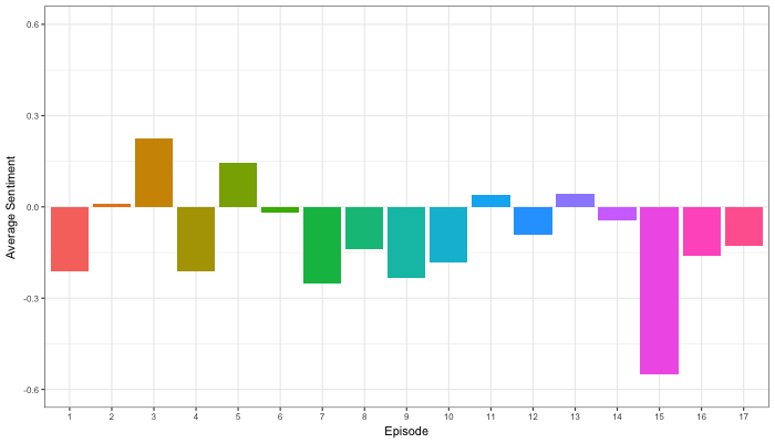
Josh Yazman did the world a favor and compared the quality of the five lexicons mentioned above. He observed their validity in relation to the millions of restaurant reviews in the Yelp dataset. This dataset includes both textual reviews and 1 to 5 star ratings. Here’s a summary of Josh’s findings, including two visualizations (read Josh’s full blog + details here):

  • NRC overestimates the positive sentiment.
  • AFINN also provides overly positive estimates, but to a lesser extent.
  • Loughran seems unreliable altogether (on Yelp data).
  • Bing estimates are accurate as long as texts are long enough (e.g., 200+ words).
  • SentiWordNet‘s estimates are mostly valid and precise, also on shorter texts, but may include minor outliers.

Sentiment scores by Yelp rating, estimated using each lexicon. [original]
The average sentiment score estimated using lexicons, where words are randomly sampled from the Yelp dataset. Note that, although both NRC and Bing scores are relatively positive on average, they also demonstrate a larger spread of scores (which is a good thing if you assume that reviews vary in terms of sentiment). [original]
On a more detailed level, David Robinson demonstrated how to uncover performance errors or quality issues in lexicons, in his 2016 blog on the AFINN lexicon. Using only the most common words (i.e., used in 200+ reviews for at least 10 businesses) of the same Yelp dataset, David visualized the inconsistencies between the AFINN sentiment lexicon and the Yelp ratings in two very smart and appealing ways:

center
Words’ AFINN sentiment score by the average rating of the reviews they used in [original]
As the figure above shows, David found a strong positive correlations between the sentiment score assigned to words in the AFINN lexicon and the way they are used in Yelp reviews. However, there are some exception – words that did not have the same meaning in the lexicon and the observed data. Examples of words that seem to cause errors are die and bomb (both negative AFINN scores but used in positive Yelp reviews) or, the other way around, joke and honor (positive AFINN scores but negative meanings on Yelp).

center
A graph of the frequency with which words are used in reviews, by the average rating of the reviews they occur in, colored for their AFINN sentiment score [original]
With the graph above, it is easy to see what words cause inaccuracies. Blue words should be in the upper section of this visual while reds should be closer to the bottom. If this is not the case, a word likely has a different meaning in the lexicon respective to how it’s used on Yelp. These lexicon-data differences become increasingly important as words are located closer to the right side of the graph, which means they more frequently screw up your sentiment estimates. For instance, fine, joke, fuck and hope cause much overestimation of positive sentiment while fresh is not considered in the positive scores it entails and die causes many negative errors.

TL;DR: Sentiment lexicons vary in terms of their quality/performance. If your texts are short (few hundred words) you might be best off using Bing (tidytext). In other cases, opt for SentiWordNet (lexicon), which considers a broader vocabulary. If possible, try to evaluate inaccuracies, outliers, and/or prediction errors via data visualizations.

Animated Snow in R

Animated Snow in R

Due to the recent updates to the gganimate package, the code below no longer produces the desired animation.
A working, updated version can be found here

After hearing R play the Jingle Bells tune, I really got into the holiday vibe. It made me think of Ilya Kashnitsky (homepage, twitter) his snowy image in R.

if(!"tidyverse" %in% installed.packages()) install.packages("tidyverse")

library("tidyverse")

n <- 100 
tibble(x = runif(n),  
y = runif(n),  
s = runif(n, min = 4, max = 20)) %>%
ggplot(aes(x, y, size = s)) +
geom_point(color = "white", pch = 42) +
scale_size_identity() +
coord_cartesian(c(0,1), c(0,1)) +
theme_void() +
theme(panel.background = element_rect("black"))

snow.png

This greatly fits the Christmas theme we have going here. Inspired by Ilya’s script, I decided to make an animated snowy GIF! Sure R is able to make something like the lively visualizations Daniel Shiffman (Coding Train) usually makes in Processing/JavaScript? It seems so:

snow

### ANIMATED SNOW === BY PAULVANDERLAKEN.COM
### PUT THIS FILE IN AN RPROJECT FOLDER

# load in packages
pkg <- c("here", "tidyverse", "gganimate", "animation")
sapply(pkg, function(x){
if (!x %in% installed.packages()){install.packages(x)}
library(x, character.only = TRUE)
})

# parameters
n <- 100 # number of flakes
times <- 100 # number of loops
xstart <- runif(n, max = 1) # random flake start x position
ystart <- runif(n, max = 1.1) # random flake start y position
size <- runif(n, min = 4, max = 20) # random flake size
xspeed <- seq(-0.02, 0.02, length.out = 100) # flake shift speeds to randomly pick from
yspeed <- runif(n, min = 0.005, max = 0.025) # random flake fall speed

# create storage vectors
xpos <- rep(NA, n * times)
ypos <- rep(NA, n * times)

# loop through simulations
for(i in seq(times)){
if(i == 1){
# initiate values
xpos[1:n] <- xstart
ypos[1:n] <- ystart
} else {
# specify datapoints to update
first_obs <- (n*i - n + 1)
last_obs <- (n*i)
# update x position
# random shift
xpos[first_obs:last_obs] <- xpos[(first_obs-n):(last_obs-n)] - sample(xspeed, n, TRUE)
# update y position
# lower by yspeed
ypos[first_obs:last_obs] <- ypos[(first_obs-n):(last_obs-n)] - yspeed
# reset if passed bottom screen
xpos <- ifelse(ypos < -0.1, runif(n), xpos) # restart at random x
ypos <- ifelse(ypos < -0.1, 1.1, ypos) # restart just above top
}
}

# store in dataframe
data_fluid <- cbind.data.frame(x = xpos,
y = ypos,
s = size,
t = rep(1:times, each = n))

# create animation
snow <- data_fluid %>%
ggplot(aes(x, y, size = s, frame = t)) +
geom_point(color = "white", pch = 42) +
scale_size_identity() +
coord_cartesian(c(0, 1), c(0, 1)) +
theme_void() +
theme(panel.background = element_rect("black"))

# save animation
gganimate(snow, filename = here("snow.gif"), title_frame = FALSE, interval = .1)

snowsnow.gifsnow.gif

Updates:

Jingle Bells in R

Jingle Bells in R

Christmas is here! Keith McNulty called on his LinkedIn network to co-create a script to play Christmas tunes. After adding some notes myself, the R script on this github page now plays Jingle Bells. The final tune you can download here and the script I pasted below. Any volunteers to make Let it snow or Silent night?

if(!"dplyr" %in% installed.packages()) install.packages("dplyr")
if(!"audio" %in% installed.packages()) install.packages("audio")

library("dplyr")
library("audio")

notes <- c(A = 0, B = 2, C = 3, D = 5, E = 7, F = 8, G = 10)

pitch <- paste("E E E",
"E E E",
"E G C D",
"E",
"F F F F",
"F E E E",
"E D D E",
"D G",
"E E E",
"E E E",
"E G C D",
"E",
"F F F F",
"F E E E E",
"G G F D",
"C",
"G3 E D C",
"G3",
"G3 G3 G3 E D C",
"A3",
"A3 F E D",
"B3",
"G G F D",
"E",
"G3 E D C",
"G3",
"G3 E D C",
"A3 A3",
"A3 F E D",
"G G G G A G F D",
"C C5 B A G F G",
"E E E G C D",
"E E E G C D",
"E F G A C E D F",
"E C D E F G A G",
"F F F F F F",
"F E E E E E",
"E D D D D E",
"D D E F G F E D",
"E E E G C D",
"E E E G C D",
"E F G A C E D F",
"E C D E F G A G",
"F F F F F F",
"F E E E E E",
"G C5 B A G F E D",
"C C E G C5")

duration <- c(1, 1, 2,
1, 1, 2,
1, 1, 1.5, 0.5,
4,
1, 1, 1, 1,
1, 1, 1, 1,
1, 1, 1, 1,
2, 2,
1, 1, 2,
1, 1, 2,
1, 1, 1.5, 0.5,
4,
1, 1, 1, 1,
1, 1, 1, 0.5, 0.5,
1, 1, 1, 1,
4,
1, 1, 1, 1,
3, .5, .5,
1, 1, 1, 1,
4,
1, 1, 1, 1,
4,
1, 1, 1, 1,
4,
1, 1, 1, 1,
4,
1, 1, 1, 1,
3, 1,
1, 1, 1, 1,
1, 1, 1, 1,
1, 1, 1, 1,
1, 0.5, 0.5, 0.5, 0.5, 0.5, 0.5,
1, 1, 0.5, 0.5, 0.5, 0.5,
1, 1, 0.5, 0.5, 0.5, 0.5,
0.5, 0.5, 0.5, 0.5, 0.5, 0.5, 0.5, 0.5,
0.5, 0.5, 0.5, 0.5, 0.5, 0.5, 0.5, 0.5,
1, 0.5, 0.5, 1, 0.5, 0.5,
1, 0.5, 0.5, 1, 0.5, 0.5,
1, 0.5, 0.5, 0.5, 0.5, 1,
1, 0.33, 0.33, 0.33, 1, 0.33, 0.33, 0.33,
1, 1, 0.5, 0.5, 0.5, 0.5,
1, 1, 0.5, 0.5, 0.5, 0.5,
0.5, 0.5, 0.5, 0.5, 0.5, 0.5, 0.5, 0.5,
0.5, 0.5, 0.5, 0.5, 0.5, 0.5, 0.5, 0.5,
1, 0.5, 0.5, 1, 0.5, 0.5,
1, 0.5, 0.5, 1, 0.5, 0.5,
0.5, 0.5, 0.5, 0.5, 0.5, 0.5, 0.5, 0.5,
1, 0.33, 0.33, 0.33, 2)

jbells <- data_frame(pitch = strsplit(pitch, " ")[[1]],
duration = duration)

jbells <- jbells %>%
mutate(octave = substring(pitch, nchar(pitch)) %>%
{suppressWarnings(as.numeric(.))} %>%
ifelse(is.na(.), 4, .),
note = notes[substr(pitch, 1, 1)],
note = note + grepl("#", pitch) -
grepl("b", pitch) + octave * 12 +
12 * (note < 3),
freq = 2 ^ ((note - 60) / 12) * 440)

tempo <- 250

sample_rate <- 44100

make_sine <- function(freq, duration) {
wave <- sin(seq(0, duration / tempo * 60, 1 / sample_rate) *
freq * 2 * pi)
fade <- seq(0, 1, 50 / sample_rate)
wave * c(fade, rep(1, length(wave) - 2 * length(fade)), rev(fade))
}

jbells_wave <- mapply(make_sine, jbells$freq, jbells$duration) %>%
do.call("c", .)

play(jbells_wave)
Sentiment Analysis of Stranger Things Seasons 1 and 2

Sentiment Analysis of Stranger Things Seasons 1 and 2

Jordan Dworkin, a Biostatistics PhD student at the University of Pennsylvania, is one of the few million fans of Stranger Things, a 80s-themed Netflix series combining drama, fantasy, mystery, and horror. Awaiting the third season, Jordan was curious as to the emotional voyage viewers went through during the series, and he decided to examine this using a statistical approach. Like I did for the seven Harry Plotter books, Jordan downloaded the scripts of all the Stranger Things episodes and conducted a sentiment analysis in R, of course using the tidyverse and tidytext. Jordan measured the positive or negative sentiment of the words in them using the AFINN dictionary and a first exploration led Jordan to visualize these average sentiment scores per episode:

The average positive/negative sentiment during the 17 episodes of the first two seasons of Stranger Things (from Medium.com)

Jordan jokingly explains that you might expect such overly negative sentiment in show about missing children and inter-dimensional monsters. The less-than-well-received episode 15 stands out, Jordan feels this may be due to a combination of its dark plot and the lack of any comedic relief from the main characters.

Reflecting on the visual above, Jordan felt that a lot of the granularity of the actual sentiment was missing. For a next analysis, he thus calculated a rolling average sentiment during the course of the separate episodes, which he animated using the animation package:

GIF displaying the rolling average (40 words) sentiment per Stranger Things episode (from Medium.com)

Jordan has two new takeaways: (1) only 3 of the 17 episodes have a positive ending – the Season 1 finale, the Season 2 premiere, and the Season 2 finale – (2) the episodes do not follow a clear emotional pattern. Based on this second finding, Jordan subsequently compared the average emotional trajectories of the two seasons, but the difference was not significant:

Smoothed (loess, I guess) trajectories of the sentiment during the episodes in seasons one and two of Stranger Things (from Medium.com)

Potentially, it’s better to classify the episodes based on their emotional trajectory than on the season they below too, Jordan thought next. Hence, he constructed a network based on the similarity (temporal correlation) between episodes’ temporal sentiment scores. In this network, the episodes are the nodes whereas the edges are weighted for the similarity of their emotional trajectories. In that sense, more distant episodes are less similar in terms of their emotional trajectory. The network below, made using igraph (see also here), demonstrates that consecutive episodes (1 → 2, 2 → 3, 3 → 4) are not that much alike:

The network of Stranger Things episodes, where the relations between the episodes are weighted for the similarity of their emotional trajectories (from Medium.com).

A community detection algorithm Jordan ran in MATLAB identified three main trajectories among the episodes:

Three different emotional trajectories were identified among the 17 Stranger Things episodes in Season 1 and 2 (from Medium.com).

Looking at the average patterns, we can see that group 1 contains episodes that begin and end with neutral emotion and have slow fluctuations in the middle, group 2 contains episodes that begin with negative emotion and gradually climb towards a positive ending, and group 3 contains episodes that begin on a positive note and oscillate downwards towards a darker ending.

– Jordan on Medium.com

Jordan final suggestion is that producers and scriptwriters may consciously introduce these variations in emotional trajectories among consecutive episodes in order to get viewers hooked. If you want to redo the analysis or reuse some of the code used to create the visuals above, you can access Jordan’s R scripts here. I, for one, look forward to his analysis of Season 3!

Association rules using FPGrowth in Spark MLlib through SparklyR

Association rules using FPGrowth in Spark MLlib through SparklyR

Great tutorial on how to conduct simple market basket analysis on your laptop either with association rules through the arules package or with frequent pattern mining (FPGrowth) in Spark via sparklyr!

Longhow Lam's avatarLonghow Lam's Blog

sparkfp

Introduction

Market Basket Analysis or association rules mining can be a very useful technique to gain insights in transactional data sets, and it can be useful for product recommendation. The classical example is data in a supermarket. For each customer we know what the individual products (items) are that he has bought. With association rules mining we can identify items that are frequently bought together. Other use cases for MBA could be web click data, log files, and even questionnaires.

In R there is a package arules to calculate association rules, it makes use of the so-called Apriori algorithm. For data sets that are not too big, calculating rules with arules in R (on a laptop) is not a problem. But when you have very huge data sets, you need to do something else, you can:

  • use more computing power (or cluster of computing nodes).
  • use another algorithm, for example…

View original post 727 more words

Facial Recognition Challenge: Chad Smith & Will Ferrell

Facial Recognition Challenge: Chad Smith & Will Ferrell

The below summarizes Part 4 of a medium.com series by Adam Geitgey.
Check out the original articles: Part 1Part 2Part 3Part 4Part 5Part 6Part 7 and Part 8!

Adam Geitgey likes to write about computers and machine learning. He explains machine learning as “generic algorithms that can tell you something interesting about a set of data without you having to write any custom code specific to the problem. Instead of writing code, you feed data to the generic algorithm and it builds its own logic based on the data.” (Part 1)


Adam’s visual explanation of two machine learning applications (original from Part 1)

In the fourth part of his series on machine learning Adam touches on Facial Recognition. Facebook is one of the companies using such algorithms in real-time, allowing them to recognize your friends’ faces after you’ve tagged them only a few times. Facebook reports they recognize faces with 97% accuracy, which is comparable to our own, human facial recognition abilities!

Facebook’s algorithms recognizing and automatically tagging Adam’s family. Helpful or creepy? (original from Part 4)


Adam decided to put up a challenge: would a facial recognition algorithm be able to distinguish Will Ferrell (famous actor) from Chad Smith (famous rock musician)? Indeed, these two celebrities look very much alike:

Image result for will ferrell chad smith
Chad Smith (left) and Will Ferell (right) on www.rollingstone.com

If you want to train such an algorithm, Adam explain, you need to overcome a series of related problems:

  1. First, look at a picture and find all the faces in it
  2. Second, focus on each face and be able to understand that even if a face is turned in a weird direction or in bad lighting, it is still the same person.
  3. Third, be able to pick out unique features of the face that you can use to tell it apart from other people— like how big the eyes are, how long the face is, etc.
  4. Finally, compare the unique features of that face to all the people you already know to determine the person’s name.

(Adam Geitgey, Part 4)


How the facial recognition algorithm steps might work (original from Part 4)

To detect the faces, Adam used Histograms of Oriented Gradients (HOG). All input pictures were converted to black and white (because color is not needed) and then every single pixel in our image is examined, one at a time. Moreover, for every pixel, the algorithm examined the pixels directly surrounding it:

Illustration of the algorithm as it would take in a black and white photo of Will Ferrel (original from Part 4)

The algorithm then checks, for every pixel, in which direction the picture is getting darker and draws an arrow (a gradient) in that direction.

Illustration of how algorithm would reduce a black and white photo of Will Ferrel to gradients (original from Part 4)

However, to do this for every single pixel would require too much processing power, so Adam broke up pictures in 16 by 16 pixel squares. The result is a very simple representation that does capture the basic structure of the original face, based on which we can now spot faces in pictures. Moreover, because we used gradients, the result will be similar regardless of the lighting of the picture.

The original image turned into a HOG representation (original from Part 4)

Now that the computer can spot faces, we need to make sure that it knows that two perspectives of the same face represent the same person. Adam uses landmarks for this: 68 specific points that exist on every face. An algorithm can then be trained to find these points on any face:

The 68 points on the image of Will Ferrell (original from Part 4)

Now the computer knows where the chin, the mouth and the eyes are, the image can be scaled and rotated to center it as best as possible:

The image of Will Ferrell transformed (original from Part 4)

Adam trained a Deep Convolutional Neural Network to generate 128 measurements for each face that best distinguish it from faces of other people. This network needs to train for several hours, going through thousands and thousands of face pictures. If you want to try this step yourself, Adam explains how to run OpenFace’s lua script. This study at Google provides more details, but it basically looks like this:

The training process visualized (original from Part 4)

After hours of training, the neural net will output 128 numbers accurately representing the specific face put in. Now, all you need to do is check which face in your database is most closely resembled by those 128 numbers, and you have your match! Many algorithms can do this final check, and Adam trained a simple linear SVM classifier on twenty pictures of Chad Smith, Will Ferrel, and Jimmy Falon (the host of a talkshow they both visited).

In the end, Adam’s machine had learned to distinguish these three people – two of whom are nearly indistinguishable with the human eye – in real-time:

Adam Geitgey’s facial recognition algorithm in action: providing real time classifications of the faces of lookalikes Chad Smith and Will Ferrel at Jimmy Falon’s talk show (original from Part 4

You can find Adam on LinkedIn, or on Twitter at @ageitgey, and I strongly recommend you examine his series on machine learning on Medium.com (Part 1). Moreover, Adam released a Python library called face_recognition, arguably easier to install and use than OpenFace, as well as a pre-configured virtual machine with face_recognition, OpenCV, TensorFlow and lots of other deep learning tools pre-installed.