Following my introduction to PCA, I will demonstrate how to apply and visualize PCA in R. There are many packages and functions that can apply PCA in R. In this post I will use the function prcomp from the stats package. I will also show how to visualize PCA in R using Base R graphics. However, my favorite visualization function for PCA is ggbiplot, which is implemented by Vince Q. Vu and available on github. Please, let me know if you have better ways to visualize PCA in R.
Computing the Principal Components (PC)
I will use the classical iris dataset for the demonstration. The data contain four continuous variables which corresponds to physical measures of flowers and a categorical variable describing the flowers’ species.
We will apply PCA to the four continuous variables and use the categorical variable to visualize the PCs later. Notice that in…
Gradient Descent is, in essence, a simple optimization algorithm. It seeks to find the gradient of a linear slope, by which the resulting linear line best fits the observed data, resulting in the smallest or lowest error(s). It is THE inner working of the linear functions we get taught in university statistics courses, however, many of us will finish our Masters (business) degree without having heard the term. Hence, this blog.
Linear regression is among the simplest and most frequently used supervised learning algorithms. It reduces observed data to a linear function (Y = a + bX) in order to retrieve a set of general rules, or to predict the Y-values for instances where the outcome is not observed.
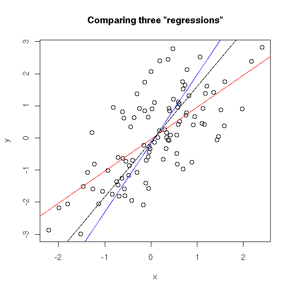
One can define various linear functions to model a set of data points (e.g. below). However, each of these may fit the data better or worse than the others. How can you determine which function fits the data best? Which function is an optimal representation of the data? Enter stage Gradient Descent. By iteratively testing values for the intersect (a; where the linear line intersects with the Y-axis (X = 0)) and the gradient (b; the slope of the line; the difference in Y when X increases with 1) and comparing the resulting predictions against the actual data, Gradient Descent finds the optimal values for the intersect and the slope. These optimal values can be found because they result in the smallest difference between the predicted values and the actual data – the least error.
The video below is part of a Coursera machine learning course of Stanford University and it provides a very intuitive explanation of the algorithm and its workings:
A recent blog demonstrates how one could program the gradient descent algorithm in R for him-/herself. Indeed, the code copied below provides the same results as the linear modelling function in R’s base environment.
gradientDesc  max_iter) {
      abline(c, m)
      converged = T
      return(paste("Optimal intercept:", c, "Optimal slope:", m))
    }
  }
}

# compare resulting coefficients
coef(lm(mpg ~ disp, data = mtcars)
gradientDesc(x = disp, y = mpg, learn_rate = 0.0000293, conv_theshold = 0.001, n = 32, max_iter = 2500000)
Although the algorithm may result in a so-called “local optimum”, representing the best fitting set of values (a & b) among a specific range of X-values, such issues can be handled but deserve a separate discussion.
A time series can be considered an ordered sequence of values of a variable at equally spaced time intervals. To model such data, one can use time series analysis (TSA). TSA accounts for the fact that data points taken over time may have an internal structure (such as autocorrelation, trend, or seasonal variation) that should be accounted for.
TSA has several purposes:
Descriptive: Identify patterns in correlated data, such as trends and seasonal variations.
Explanation: These patterns may help in obtaining an understanding of the underlying forces and structure that produced the data.
Forecasting: In modelling the data, one may obtain accurate predictions of future (short-term) trends.
Intervention analysis: One can examine how (single) events have influenced the time series.
Quality control: Deviations on the time series may indicate problems in the process reflected by the data.
TSA has many applications, including:
Economic Forecasting
Sales Forecasting
Budgetary Analysis
Stock Market Analysis
Yield Projections
Process and Quality Control
Inventory Studies
Workload Projections
Utility Studies
Census Analysis
Strategic Workforce Planning
AlgoBeans has a nice tutorial on implementing a simple TS model in Python. They explain and demonstrate how to deconstruct a time series into daily, weekly, monthly, and yearly trends, how to create a forecasting model, and how to validate such a model.
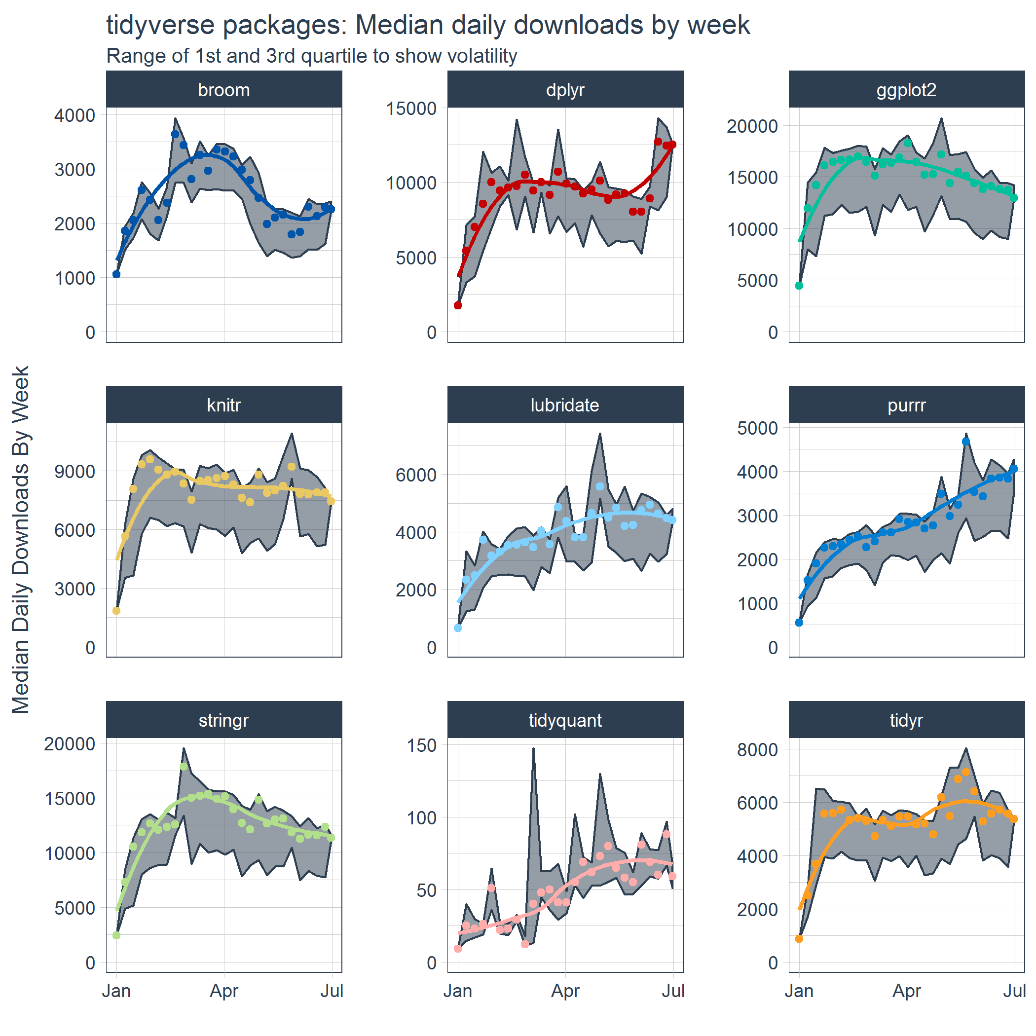
Analytics Vidhya hosts a more comprehensive tutorial on TSA in R. They elaborate on the concepts of a random walk and stationarity, and compare autoregressive and moving average models. They also provide some insight into the metrics one can use to assess TS models. This web-tutorial runs through TSA in R as well, showing how to perform seasonal adjustments on the data. Although the datasets they use have limited practical value (for businesses), the stepwise introduction of the different models and their modelling steps may come in handy for beginners. Finally, business-science.io has three amazing posts on how to implement time series in R following the tidyverse principles using the tidyquant package (Part 1; Part 2; Part 3; Part 4).
Statistical literacy is essential to our data-driven society. Analytics has been and continues to be a game changer in many business fields, among other Human Resources. Yet, for all the increased importance and demand for statistical competence, the pedagogical approaches in statistics have barely changed.
Seeing Theory is a project designed and created by Daniel Kunin with support from Brown University’s Royce Fellowship Program. The goal of the project is to make statistics more accessible to a wider range of students through interactive visualizations.
Using JavaScript, the researchers have made statistics both intuitive and beautiful at the same time.
Veritasium makes educational video’s, mostly about science, and recently they recorded one offering an intuitive explanation of Bayes’ Theorem. They guide the viewer through Bayes’ thought process coming up with the theory, explain its workings, but also acknowledge some of the issues when applying Bayesian statistics in society.
“The thing we forget in Bayes’ Theorem is that our actions play a role in determining outcomes, in determining how true things actually are.” 8.23
“A really good understanding of Bayes’ Theorem implies that experimentation is essential: if you’ve been doing the same thing for a long time and getting the same result – that you’re not necessarily happy with – maybe it’s time to change.” 8.48