Tag: textmining

Wordle with NLP for Data Scientists

I have played my fair share of Wordle.

I’m not necessarily good at it, but most days I get to solve the puzzle.

The experience is completely different with Semantle — a Wordle-inspired puzzle in which you also need to guess the word of the day.

Unlike in Wordle, Semantle gives you unlimited guesses though. And, boy, you will need many!

Like Wordle, Semantle gives you hints as to how close your guesses were to the secret word of the day.

However, where Wordle shows you how good your guesses were in terms of the letters used, Semantle evaluates the semantic similarity of your guesses to the secret word. For the 1000 most similar words to the secret word, it will show you its closeness like in the picture above.

This semantic similarity comes from the domain of Natural Language Processing — NLP — and this basically reflects how often words are used in similar contexts in natural language.

For instance, the words “love” and “hate” may seem like opposites, but they will often score similarly in grammatical sentences. According to the semantle FAQ the actual opposite of “love” is probably something like “Arizona Diamondbacks”, or “carburetor”.

Another example is last day’s solution (15 March 2022), when the secret word was circle. The ten closest words you could have guessed include circles and semicircle, but more distinctive words such as corner and clockwise.

Further downfield you could have guessed relatively close words like saucer, dot, parabola, but I would not have expected words like outwaited, weaved, and zipped.

The creator of Semantle scored the semantic similarity for almost all words used in the English language, by training a so-called word2vec model based on a very large dataset of news articles (GoogleNews-vectors-negative300.bin from late 2021).

Now, every day, one word is randomly selected as the secret word, and you can try to guess which one it is. I usually give up after 300 to 400 guesses, but my record was 76 guesses for uncovering the secret word world.

Try it out yourself: https://semantle.novalis.org/

And do share your epic wins and fails!

Chatterplots

I’ve mentioned before that I dislike wordclouds (for instance here, or here) and apparently others share that sentiment. In his recent Medium blog, Daniel McNichol goes as far as to refer to the wordcloud as the pie chart of text data! Among others, Daniel calls wordclouds disorienting, one-dimensional, arbitrary and opaque and he mentions their lack of order, information, and scale.

Wordcloud of the negative characteristics of wordclouds, via Medium

Instead of using wordclouds, Daniel suggests we revert to alternative approaches. For instance, in their Tidy Text Mining with R book, Julia Silge and David Robinson suggest using bar charts or network graphs, providing the necessary R code. Another alternative is provided in Daniel’s blog: the chatterplot!

While Daniel didn’t invent this unorthodox wordcloud-like plot, he might have been the first to name it a chatterplot. Daniel’s chatterplot uses a full x/y cartesian plane, turning the usually only arbitrary though exploratory wordcloud into a more quantitatively sound, information-rich visualization.

R package ggplot’s geom_text() function — or alternatively ggrepel‘s geom_text_repel() for better legibility — is perfectly suited for making a chatterplot. And interesting features/variables for the axis — apart from the regular word frequencies — can be easily computed using the R tidytext package.

Here’s an example generated by Daniel, plotting words simulatenously by their frequency of occurance in comments to Hacker News articles (y-axis) as well as by the respective popularity of the comments the word was used in (log of the ranking, on the x-axis).

[CHATTERPLOTs are] like a wordcloud, except there’s actual quantitative logic to the order, placement & aesthetic aspects of the elements, along with an explicit scale reference for each. This allows us to represent more, multidimensional information in the plot, & provides the viewer with a coherent visual logic& direction by which to explore the data.
Daniel McNichol via Medium

I highly recommend the use of these chatterplots over their less-informative wordcloud counterpart, and strongly suggest you read Daniel’s original blog, in which you can also find the R code for the above visualizations.

Become a data-driven Sommelier by text mining wine reviews

Aleszu Bajak at Storybench.org published a great demonstration of the power of text mining. He used the R tidytext package to analyse 150,000 wine reviews which Zach Thoutt had scraped from Wine Enthusiast in November of 2017.

Aleszu started his analysis on only the French wines, with a simple word count per region:

Next, he applied TF-IDF to surface the words that are most characteristic for specific French wine regions — words used often in combination with that specific region, but not in relation to other regions.

The data also contained some price information, which Aleszu mapped France with ggplot2 and the maps package to demonstrate which French wine regions are generally more costly.

On the full dataset, Alezsu also demonstrated that there is a strong relationship between price and points, meaning that, in general, more expensive wines seem to get better reviews:

The full script and more details you can find in the orginal blog.

Identifying “Dirty” Twitter Bots with R and Python

Past week, I came across two programming initiatives to uncover Twitter bots and one attempt to identify fake Instagram accounts.

Mike Kearney developed the R package botornot which applies machine learning to estimate the probability that a Twitter user is a bot. His default model is a gradient boosted model trained using both users-level (bio, location, number of followers and friends, etc.) and tweets-level information (number of hashtags, mentions, capital letters, etc.). This model is 93.53% accurate when classifying bots and 95.32% accurate when classifying non-bots. His faster model uses only the user-level data and is 91.78% accurate when classifying bots and 92.61% accurate when classifying non-bots. Unfortunately, the models did not classify my account correctly (see below), but you should definitely test yourself and your friends via this Shiny application.

Fun fact: botornot can be integrated with Mike’s rtweet package

Scraping Dirty Bots

At around the same time, I read this very interesting blog by Andy Patel. Annoyed by the fake Twitter accounts that kept liking and sharing his tweets, Andy wrote a Python script called pronbot_search. It’s an iterative search algorithm which Andy seeded with the dozen fake Twitter accounts that he identified originally. Subsequently, the program iterated over the friends and followers of each of these fake users, looking for other accounts displaying similar traits (e.g., similar description, including an URL to a sex-website called “Dirty Tinder”).

Whenever a new account was discovered, it was added to the query list, and the process continued. Because of the Twitter API restrictions, the whole crawling process took literal days before Andy manually terminated it. The results are just amazing:

After a day, the results looked like so. Notice the weird clusters of relationships in this network. [original]

The full bot network uncovered by Andy included 22.000 fake Twitter accounts:

At the end of the weekend of March 10th, Andy had to stop the scraper after running for several days even though he had only processed 18% of the networks of the 22.000 included Twitter bots [original]

The bot network on Twitter is probably enormous! Zooming in on the network, Andy notes that:

Pretty much the same pattern I’d seen after one day of crawling still existed after one week. Just a few of the clusters weren’t “flower” shaped.

Andy Patel, March 2018, link

Zoomed in to a specific part of the network you can see the separate clusters of bots doing little more than liking each others messages. [original]

In his blog, Andy continues to look at all kind of data on these fake accounts. I found most striking that many of these account are years and years old already. Potentially, Twitter can use Mike Kearney’s botornot application to spot and remove them!

Most of the bots in the Dirty Tinder network found by Andy Patel were 3 to 8 years old already. [original]

Andy was nice enough to share the data on these bot accounts here, for you to play with. His Python code is stored in the same github repo and more details around this project you can read in his original blog.

Fake Instagram Accounts

Finally, SRFdata (Timo Grossenbacher) attempted to uncover fake Instagram followers among the 7 million followers in the network of 115 important Swiss Instagram influencers in R. Magi Metrics was used to retrieve information for public Instagram accounts and rvest for private accounts. Next, clear fake accounts (e.g., little followers, following many, no posts, no profile picture, numbers in name) were labelled manually, and approximately 10% of the inspected 1000 accounts appeared fake. Finally, they trained a random forest model to classify fake accounts with a sensitivity (true negative) rate of 77.4% and an overall accuracy of around 94%.

Harry Plotter: Network analysis of spell usage

Apparently, I was not the only geek who decided to celebrate the 20th anniversary of the Harry Potter saga with statistical analysis. Students Moritz Haine and Markus Dienstknecht of the Data Science for Decision Making Master at Maastricht University started their own celebratory project as part of a course Information Retrieval and Text Mining.

Students in previous years looked at for example Lord of the Rings, Star Wars and Game of Thrones. However, to our surprise, Harry Potter was missing. Since the books are about magic, we decided it would be interesting to identify all of the spells and the wizards that cast the most spells

Moritz Haine

From the books, the students extracted 41 different wizards, 64 different spells and 253 spells. Moritz points out that they could only include spoken spells, even though the most powerful wizards can also cast spells without naming them. They expect this might be the reason why Dumbledore and Voldemort are not ranked as high. At the end of their project, Moritz and Markus visualized their results in a spell-character mapping.

This is the latest addition to my collection of Harry Potter analyses, to which a similar, interactive web application of spell usage was added only last week.

Harry Plotter: Shiny App of Spell Usage

In my second Harry Plotter blog (22-Aug-2017), I wrote:

I would like to demonstrate how regular expressions can be used to retrieve (sub)strings that follow a specific format. We could use regex to examine, for instance, when, and by whom, which magical spells are cast.

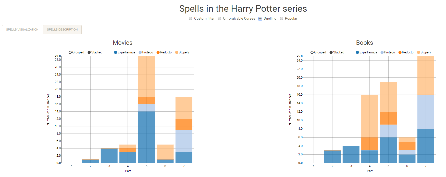
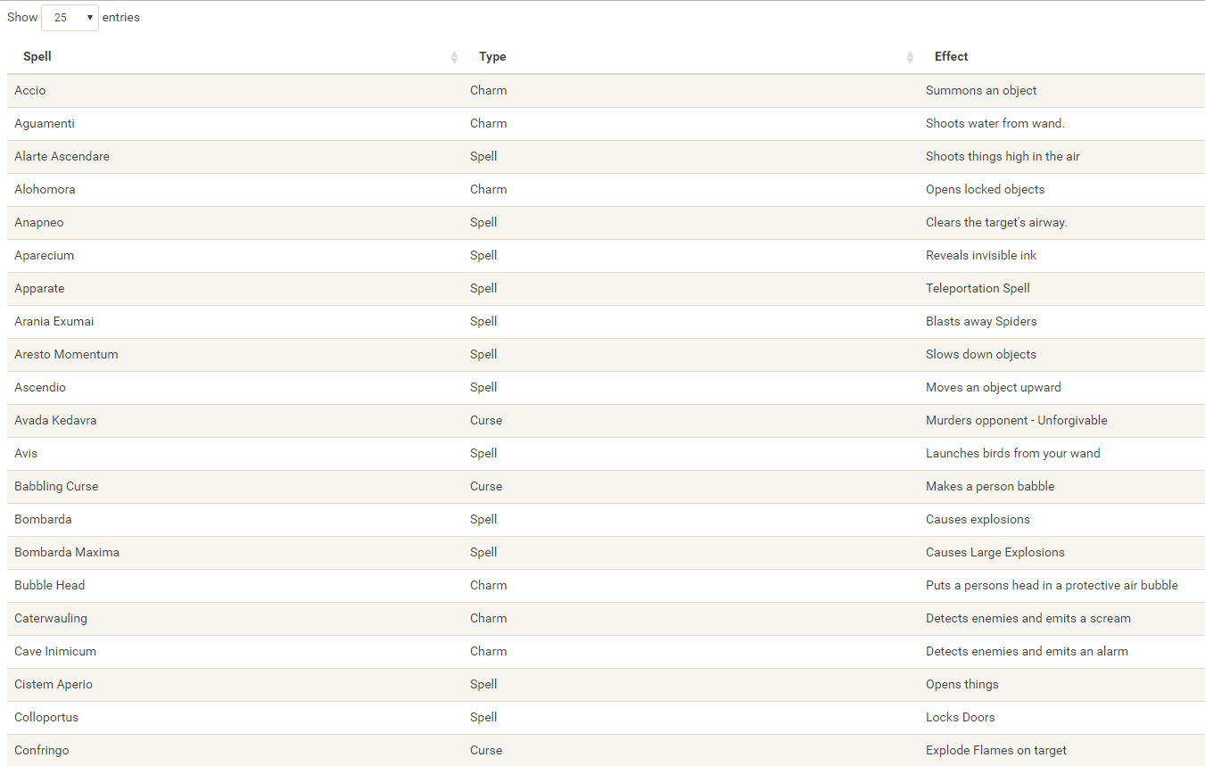
Well, Prusinowskik (real name unknown) beat me to it, and how! S/He formed a comprehensive list of all spells found in the Harry Potter saga (see below), and categorized these into “spells“, “charms“, and “curses“, and into “popular“, “dueling” and “unforgivable” purposes. Next, Prusinowskik built an interactive Shiny application with lovely JavaScript graphs (package: rCharts) for us to discover precisely when during the saga which spells are cast (see also below). Moreover, the analysis was repeated for both the books and the movies.

Truly excellent work Prusinowskik! The Shiny app can be found here.