Tag: neuralnetwork

Using OpenCV to win Mobile games

OpenCV is open-source library with tools and functionalities that support computer vision. It allows your computer to use complex mathematics to detect lines, shapes, colors, text and what not.

OpenCV was originally developed by Intel in 2000 and sometime later someone had the bright idea to build a Python module on top of it.

Using a simple…

pip install opencv-python

…you can now use OpenCV in Python to build advanced computer vision programs.

And this is exactly what many professional and hobby programmers are doing. Specifically, to get their computer to play (and win) mobile app games.

ZigZag

In ZigZag, you are a ball speeding down a narrow pathway and your only mission is to avoid falling off.

Using OpenCV, you can get your computer to detect objects, shapes, and lines.

This guy set up an emulator on his computer, so the computer can pretend to be a mobile device. Then he build a program using Python’s OpenCV module to get a top score

You can find the associated code here, but note that will need to set up an emulator yourself before being able to run this code.

Kick Ya Chop

In Kick Ya Chop, you need to stomp away parts of a tree as fast as you can, without hitting any of the branches.

This guy uses OpenCV to perform image pattern matching to allow his computer to identify and avoid the trees braches. Find the code here.

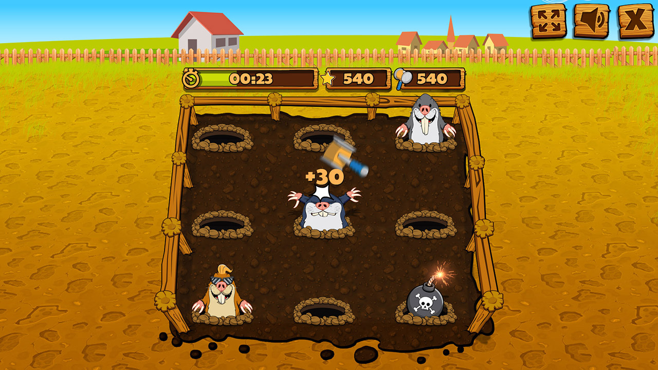
Whack ‘Em All

We all know how to play Whack a Mole, and now this computer knows how to too. Code here.

Pong

This last game also doesn’t need an introduction, and you can find the code here.

Is this machine learning or AI?

If you’d ask me, the videos above provide nice examples of advanced automation. But there’s no real machine learning or AI involved.

Yes, sure, the OpenCV package uses pre-trained neural networks under the hood, and you can definitely call those machine learning. But the programmers who now use the opencv library just leverage the knowledge stored in those network to create very basal decision rules.

IF pixel pattern of mole
THEN whack!
ELSE no whack.

To me, it’s only machine learning when there’s really some learning going on. A feedback loop with performance improvement. And you may call it AI, IMO, when the feedback loop is more or less autonomous.

Fortunately, programmers have also been taking a machine learning/AI approach to beating games. Specifically using reinforcement learning. Think of famous applications like AlphaGo and AlphaStar. But there are also hobby programmers who use similar techniques. For example, to get their computer to obtain highscores on Trackmania.

In a later post, I’ll dive into those in more detail.

Tutorial: Demystifying Deep Learning for Data Scientists

In this great tutorial for PyCon 2020, Eric Ma proposes a very simple framework for machine learning, consisting of only three elements:

Model
Loss function
Optimizer

Screenshot from youtube.com/watch?v=gGu3pPC_fBM

By adjusting the three elements in this simple framework, you can build any type of machine learning program.

In the tutorial, Eric shows you how to implement this same framework in Python (using jax) and implement linear regression, logistic regression, and artificial neural networks all in the same way (using gradient descent).

I can’t even begin to explain it as well as Eric does himself, so I highly recommend you watch and code along with the Youtube tutorial (~1 hour):

If you want to code along, here’s the github repository: github.com/ericmjl/dl-workshop

Have you ever wondered what goes on behind the scenes of a deep learning framework? Or what is going on behind that pre-trained model that you took from Kaggle? Then this tutorial is for you! In this tutorial, we will demystify the internals of deep learning frameworks – in the process equipping us with foundational knowledge that lets us understand what is going on when we train and fit a deep learning model. By learning the foundations without a deep learning framework as a pedagogical crutch, you will walk away with foundational knowledge that will give you the confidence to implement any model you want in any framework you choose.
https://www.youtube.com/watch?v=gGu3pPC_fBM

Via github.com/ericmjl/dl-workshop/blob/master/docs/figures/linreg-neural.png

An ABC of Artificial Intelligence Concepts

Yet another great resource by one of the teams at Google in collaboration with Oxford:

An ABC of Artificial Intelligence-related concepts!

The G is for GANs: Generative Adverserial Networks.

Via atozofai.withgoogle.com/intl/en-GB/gans/

Want to know what GANs are all about?

Just read along with Google’s laymen explanation! Here’s an excerpt:

The P is for Predictions.

Via atozofai.withgoogle.com/intl/en-US/predictions/

Currently the ABC is only available in English, but other language translations come available soon.

Check it out yourself!

Making Pictures 3D using Context-aware Layered Depth Inpainting

Several Chinese Ph.D. students wrote a PyTorch program that can turn your holiday pictures into 3D sceneries. They call it 3D photo inpainting. Here are some examples

And here’s the new method compares to previous techniques:

Here are several links to more detailed resources: [Paper] [Project Website] [Google Colab] [GitHub]

We propose a method for converting a single RGB-D input image into a 3D photo, i.e., a multi-layer representation for novel view synthesis that contains hallucinated color and depth structures in regions occluded in the original view. We use a Layered Depth Image with explicit pixel connectivity as underlying representation, and present a learning-based inpainting model that iteratively synthesizes new local color-and-depth content into the occluded region in a spatial context-aware manner. The resulting 3D photos can be efficiently rendered with motion parallax using standard graphics engines. We validate the effectiveness of our method on a wide range of challenging everyday scenes and show fewer artifacts when compared with the state-of-the-arts.
Via github.com/vt-vl-lab/3d-photo-inpainting

3D Photography Inpainting: Exploring Art with AI. - Towards Data ... — I loved this one as well, but it could be a different technique used, via Medium

AutoML-Zero: Evolving Machine Learning Algorithms From Scratch

Google Brain researchers published this amazing paper, with accompanying GIF where they show the true power of AutoML.

AutoML stands for automated machine learning, and basically refers to an algorithm autonomously building the best machine learning model for a given problem.

This task of selecting the best ML model is difficult as it is. There are many different ML algorithms to choose from, and each of these has many different settings ([hyper]parameters) you can change to optimalize the model’s predictions.

For instance, let’s look at one specific ML algorithm: the neural network. Not only can we try out millions of different neural network architectures (ways in which the nodes and lyers of a network are connected), but each of these we can test with different loss functions, learning rates, dropout rates, et cetera. And this is only one algorithm!

In their new paper, the Google Brain scholars display how they managed to automatically discover complete machine learning algorithms just using basic mathematical operations as building blocks. Using evolutionary principles, they have developed an AutoML framework that tailors its own algorithms and architectures to best fit the data and problem at hand.

This is AI research at its finest, and the results are truly remarkable!

GIF for the interpretation of the best evolved algorithm

You can read the full paper open access here: https://arxiv.org/abs/2003.03384 (quick download link)

The original code is posted here on github: github.com/google-research/google-research/tree/master/automl_zero#automl-zero

Building a realistic Reddit AI that get upvoted in Python

Sometimes I find these AI / programming hobby projects that I just wished I had thought of…

Will Stedden combined OpenAI’s GPT-2 deep learning text generation model with another deep-learning language model by Google called BERT (Bidirectional Encoder Representations from Transformers) and created an elaborate architecture that had one purpose: posting the best replies on Reddit.

The architecture is shown at the end of this post — copied from Will’s original blog here. Moreover, you can read this post for details regarding the construction of the system. But let me see whether I can explain you what it does in simple language.

The below is what a Reddit comment and reply thread looks like. We have str8cokane making a comment to an original post (not in the picture), and then tupperware-party making a reply to that comment, followed by another reply by str8cokane. Basically, Will wanted to create an AI/bot that could write replies like tupperware-party that real people like str8cokane would not be able to distinguish from “real-people” replies.

Note that with 4 points, str8cokane‘s original comments was “liked” more than tupperware-party‘s reply and str8cokane‘s next reply, which were only upvoted 2 and 1 times respectively.

gpt2-bert on China — Example reddit comment and replies (via bonkerfield.org/)

So here’s what the final architecture looks like, and my attempt to explain it to you.

Basically, we start in the upper left corner, where Will uses a database (i.e. corpus) of Reddit comments and replies to fine-tune a standard, pretrained GPT-2 model to get it to be good at generating (red: “fake”) realistic Reddit replies.
Next, in the upper middle section, these fake replies are piped into a standard, pretrained BERT model, along with the original, real Reddit comments and replies. This way the BERT model sees both real and fake comments and replies. Now, our goal is to make replies that are undistinguishable from real replies. Hence, this is the task the BERT model gets. And we keep fine-tuning the original GPT-2 generator until the BERT discriminator that follows is no longer able to distinguish fake from real replies. Then the generator is “fooling” the discriminator, and we know we are generating fake replies that look like real ones!
You can find more information about such generative adversarial networks here.
Next, in the top right corner, we fine-tune another BERT model. This time we give it the original Reddit comments and replies along with the amount of times they were upvoted (i.e. sort of like likes on facebook/twitter). Basically, we train a BERT model to predict for a given reply, how much likes it is going to get.
Finally, we can go to production in the lower lane. We give a real-life comment to the GPT-2 generator we trained in the upper left corner, which produces several fake replies for us. These candidates we run through the BERT discriminator we trained in the upper middle section, which determined which of the fake replies we generated look most real. Those fake but realistic replies are then input into our trained BERT model of the top right corner, which predicts for every fake but realistic reply the amount of likes/upvotes it is going to get. Finally, we pick and reply with the fake but realistic reply that is predicted to get the most upvotes!

What Will’s final architecture, combining GPT-2 and BERT, looked like (via bonkerfield.org)

The results are astonishing! Will’s bot sounds like a real youngster internet troll! Do have a look at the original blog, but here are some examples. Note that tupperware-party — the Reddit user from the above example — is actually Will’s AI.

COMMENT: 'Dune’s fandom is old and intense, and a rich thread in the cultural fabric of the internet generation' BOT_REPLY:'Dune’s fandom is overgrown, underfunded, and in many ways, a poor fit for the new, faster internet generation.'

bot responds to specific numerical bullet point in source comment

Will ends his blog with a link to the tutorial if you want to build such a bot yourself. Have a try!

Moreover, he also notes the ethical concerns:

I know there are definitely some ethical considerations when creating something like this. The reason I’m presenting it is because I actually think it is better for more people to know about and be able to grapple with this kind of technology. If just a few people know about the capacity of these machines, then it is more likely that those small groups of people can abuse their advantage.
I also think that this technology is going to change the way we think about what’s important about being human. After all, if a computer can effectively automate the paper-pushing jobs we’ve constructed and all the bullshit we create on the internet to distract us, then maybe it’ll be time for us to move on to something more meaningful.
If you think what I’ve done is a problem feel free to email me , or publically shame me on Twitter.
Will Stedden via bonkerfield.org/2020/02/combining-gpt-2-and-bert/