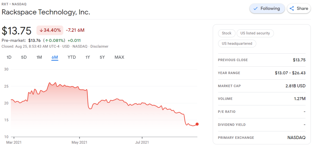
Obviously, this is less than ideal for me, but also, I should not be surprised.
Clearly, I knew nothing about the company I bought shares in. Apparently they are going through some big time reorganization, and this is not good price-wise.
According to Investopedia: A quarterly report is a summary or collection of unaudited financial statements, such as balance sheets, income statements, and cash flow statements, issued by companies every quarter (three months). In addition to reporting quarterly figures, these statements may also provide year-to-date and comparative (e.g., last year’s quarter to this year’s quarter) results. Publicly-traded companies must file their reports with the Securities Exchange Committee (SEC).
Fortunately these quarterly reports are readily available on the investors relation page, and they are not that hard to read once you have seen a few.
Visualizing financial data
I was excited to see that Rackspace offered their financial performance in bite-sized bits to me as a laymen, through their usage of nice visualizations of the financial data.
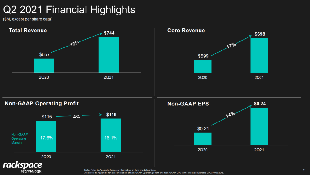
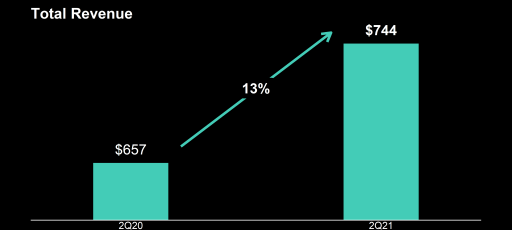
Please take a moment to process the below copy of page 11 of their 2021 Q2 report:
Though… the longer I looked at these charts… the more my head started to hurt…
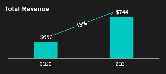
How can the growth line be about the same in the three charts Total Revenue (top-left), Core Revenue (top-right), and Non-GAAP EPS (bottom-right)? They represent different increments: 13%, 17%, and 14% respectively.
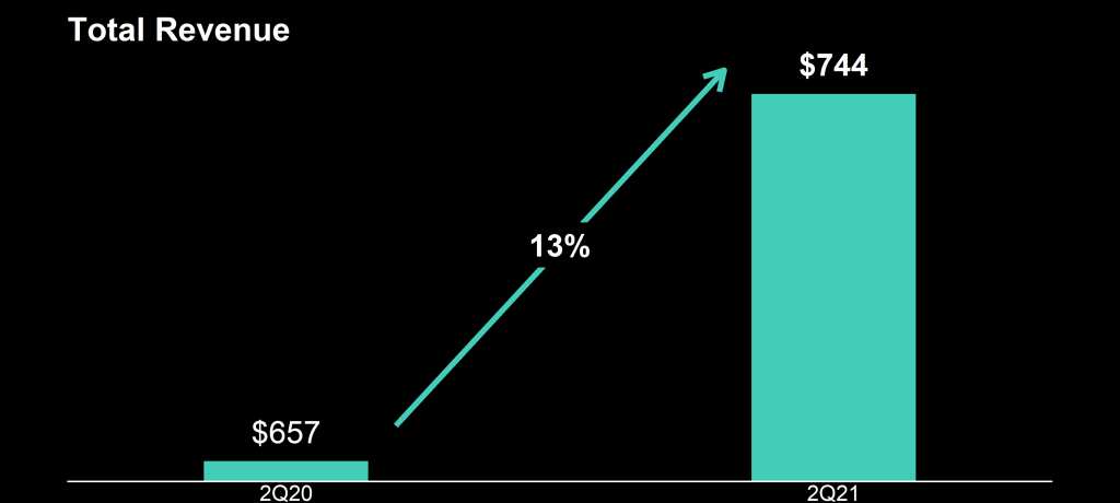
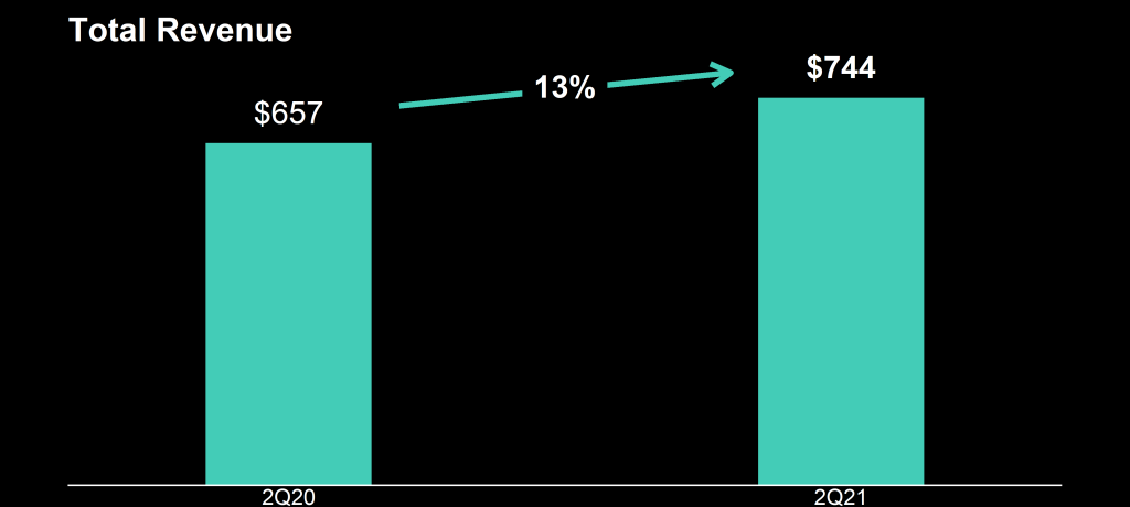
Zooming in on the top left: how does the $657 revenue of 2Q20 fit inside the $744 revenue of 2Q21 almost three times?!
Grant McDermott developed this new R package I wish I had thought of: parttree
parttree includes a set of simple functions for visualizing decision tree partitions in R with ggplot2. The package is not yet on CRAN, but can be installed from GitHub using:
Using the familiar ggplot2 syntax, we can simply add decision tree boundaries to a plot of our data.
In this example from his Github page, Grant trains a decision tree on the famous Titanic data using the parsnip package. And then visualizes the resulting partition / decision boundaries using the simple function geom_parttree()
library(parsnip)
library(titanic) ## Just for a different data set
set.seed(123) ## For consistent jitter
titanic_train$Survived = as.factor(titanic_train$Survived)
## Build our tree using parsnip (but with rpart as the model engine)
ti_tree =
  decision_tree() %>%
  set_engine("rpart") %>%
  set_mode("classification") %>%
  fit(Survived ~ Pclass + Age, data = titanic_train)
## Plot the data and model partitions
titanic_train %>%
  ggplot(aes(x=Pclass, y=Age)) +
  geom_jitter(aes(col=Survived), alpha=0.7) +
  geom_parttree(data = ti_tree, aes(fill=Survived), alpha = 0.1) +
  theme_minimal()
Super awesome!
This visualization precisely shows where the trained decision tree thinks it should predict that the passengers of the Titanic would have survived (blue regions) or not (red), based on their age and passenger class (Pclass).
This will be super helpful if you need to explain to yourself, your team, or your stakeholders how you model works. Currently, only rpart decision trees are supported, but I am very much hoping that Grant continues building this functionality!
For instance, if you’re making multiple plots of the dataset — say a group of 5 companies — you want to have each company have the same, consistent coloring across all these plots.
R has some great data visualization capabilities. Particularly the ggplot2 package makes it so easy to spin up a good-looking visualization quickly.
The default in R is to look at the number of groups in your data, and pick “evenly spaced” colors across a hue color wheel. This looks great straight out of the box:
# install.packages('ggplot2')
library(ggplot2)

theme_set(new = theme_minimal()) # sets a default theme

set.seed(1) # ensure reproducibility

# generate some data
n_companies = 5
df1 = data.frame(
  company = paste('Company', seq_len(n_companies), sep = '_'),
  employees = sample(50:500, n_companies),
  stringsAsFactors = FALSE
)

# make a simple column/bar plot
ggplot(data = df1) +
  geom_col(aes(x = company, y = employees, fill = company))
However, it can be challenging is to make coloring consistent across plots.
For instance, suppose we want to visualize a subset of these data points.
index_subset1 = c(1, 3, 4, 5) # specify a subset

# make a plot using the subsetted dataframe
ggplot(data = df1[index_subset1, ]) +
  geom_col(aes(x = company, y = employees, fill = company))
As you can see the color scheme has now changed. With one less group / company, R now picks 4 new colors evenly spaced around the color wheel. All but the first are different to the original colors we had for the companies.
One way to deal with this in R and ggplot2, is to add a scale_* layer to the plot.
Here we manually set Hex color values in the scale_fill_manual function. These hex values I provided I know to be the default R values for four groups.
# install.packages('scales')

# the hue_pal function from the scales package looks up a number of evenly spaced colors
# which we can save as a vector of character hex values
default_palette = scales::hue_pal()(5)

# these colors we can then use in a scale_* function to manually override the color schema
ggplot(data = df1[index_subset1, ]) +
  geom_col(aes(x = company, y = employees, fill = company)) +
  scale_fill_manual(values = default_palette[-2]) # we remove the element that belonged to company 2
As you can see, the colors are now aligned with the previous schema. Only Company 2 is dropped, but all other companies retained their color.
However, this was very much hard-coded into our program. We had to specify which company to drop using the default_palette[-2].
If the subset changes, which often happens in real life, our solution will break as the values in the palette no longer align with the groups R encounters:
index_subset2 = c(1, 2, 5) # but the subset might change

# and all manually-set colors will immediately misalign
ggplot(data = df1[index_subset2, ]) +
  geom_col(aes(x = company, y = employees, fill = company)) +
  scale_fill_manual(values = default_palette[-2])
Fortunately, R is a smart language, and you can work your way around this!
All we need to do is created, what I call, a named-color palette!
It’s as simple as specifying a vector of hex color values! Alternatively, you can use the grDevices::rainbow or grDevices::colors() functions, or one of the many functions included in the scales package
# you can hard-code a palette using color strings
c('red', 'blue', 'green')

# or you can use the rainbow or colors functions of the grDevices package
rainbow(n_companies)
colors()[seq_len(n_companies)]

# or you can use the scales::hue_pal() function
palette1 = scales::hue_pal()(n_companies)
print(palette1)
Now we need to assign names to this vector of hex color values. And these names have to correspond to the labels of the groups that we want to colorize.
With this named color vector and the scale_*_manual functions we can now manually override the fill and color schemes in a flexible way. This results in the same plot we had without using the scale_*_manual function:
ggplot(data = df1) +
  geom_col(aes(x = company, y = employees, fill = company)) +
  scale_fill_manual(values = palette1_named)
However, now it does not matter if the dataframe is subsetted, as we specifically tell R which colors to use for which group labels by means of the named color palette:
# the colors remain the same if some groups are not found
ggplot(data = df1[index_subset1, ]) +
  geom_col(aes(x = company, y = employees, fill = company)) +
  scale_fill_manual(values = palette1_named)
# and also if other groups are not found
ggplot(data = df1[index_subset2, ]) +
  geom_col(aes(x = company, y = employees, fill = company)) +
  scale_fill_manual(values = palette1_named)
Once you are aware of these superpowers, you can do so much more with them!
How about highlighting a specific group?
Just set all the other colors to ‘grey’…
# lets create an all grey color palette vector
palette2 = rep('grey', times = n_companies)
palette2_named = setNames(object = palette2, nm = df1$company)
print(palette2_named)
# this looks terrible in a plot
ggplot(data = df1) +
  geom_col(aes(x = company, y = employees, fill = company)) +
  scale_fill_manual(values = palette2_named)
… and assign one of the company’s colors to be a different color
# override one of the 'grey' elements using an index by name
palette2_named['Company_2'] = 'red'
print(palette2_named)
# and our plot is professionally highlighting a certain group
ggplot(data = df1) +
  geom_col(aes(x = company, y = employees, fill = company)) +
  scale_fill_manual(values = palette2_named)
We can apply these principles to other types of data and plots.
For instance, let’s generate some time series data…
timepoints = 10
df2 = data.frame(
  company = rep(df1$company, each = timepoints),
  employees = rep(df1$employees, each = timepoints) + round(rnorm(n = nrow(df1) * timepoints, mean = 0, sd = 10)),
  time = rep(seq_len(timepoints), times = n_companies),
  stringsAsFactors = FALSE
)
… and visualize these using a line plot, adding the color palette in the same way as before:
ggplot(data = df2) +
  geom_line(aes(x = time, y = employees, col = company), size = 2) +
  scale_color_manual(values = palette1_named)
If we miss one of the companies — let’s skip Company 2 — the palette makes sure the others remained colored as specified:
ggplot(data = df2[df2$company %in% df1$company[index_subset1], ]) +
  geom_line(aes(x = time, y = employees, col = company), size = 2) +
  scale_color_manual(values = palette1_named)
Also the highlighted color palete we used before will still work like a charm!
ggplot(data = df2) +
  geom_line(aes(x = time, y = employees, col = company), size = 2) +
  scale_color_manual(values = palette2_named)
Now, let’s scale up the problem! Pretend we have not 5, but 20 companies.
The code will work all the same!
set.seed(1) # ensure reproducibility

# generate new data for more companies
n_companies = 20
df1 = data.frame(
  company = paste('Company', seq_len(n_companies), sep = '_'),
  employees = sample(50:500, n_companies),
  stringsAsFactors = FALSE
)

# lets create an all grey color palette vector
palette2 = rep('grey', times = n_companies)
palette2_named = setNames(object = palette2, nm = df1$company)

# highlight one company in a different color
palette2_named['Company_2'] = 'red'
print(palette2_named)

# make a bar plot
ggplot(data = df1) +
  geom_col(aes(x = company, y = employees, fill = company)) +
  scale_fill_manual(values = palette2_named) +
  theme(axis.text.x = element_text(angle = 45, hjust = 1, vjust = 1)) # rotate and align the x labels
Also for the time series line plot:
timepoints = 10
df2 = data.frame(
  company = rep(df1$company, each = timepoints),
  employees = rep(df1$employees, each = timepoints) + round(rnorm(n = nrow(df1) * timepoints, mean = 0, sd = 10)),
  time = rep(seq_len(timepoints), times = n_companies),
  stringsAsFactors = FALSE
)

ggplot(data = df2) +
  geom_line(aes(x = time, y = employees, col = company), size = 2) +
  scale_color_manual(values = palette2_named)
The possibilities are endless; the power is now yours!
Just think at the efficiency gain if you would make a custom color palette, with for instance your company’s brand colors!
For more R tricks to up your programming productivity and effectiveness, visit the R tips and tricks page!
However, paletteer is by far my favorite package for customizing your colors in R!
The paletteer package offers direct access to 1759 color palettes, from 50 different packages!
After installing and loading the package, paletteer works as easy as just adding one additional line of code to your ggplot:
install.packages("paletteer")
library(paletteer)

install.packages("ggplot2")
library(ggplot2)

ggplot(iris, aes(Sepal.Length, Sepal.Width, color = Species)) +
  geom_point() +
  scale_color_paletteer_d("nord::aurora")
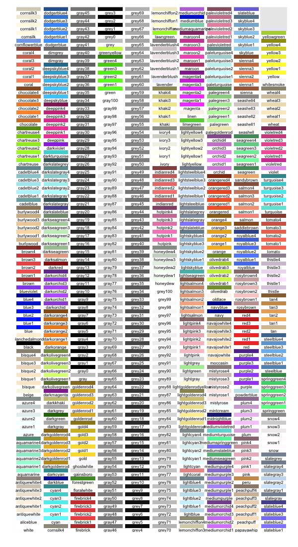
paletteer offers a combined collection of hundreds of other color palettes offered in the R programming environment, so you are sure you will find a palette that you like! Here’s the list copied below, but this github repo provides more detailed information about the package contents.
Most of my data visualizations I create using R programming — as you might have noticed from the content of my website.
Though I am colorblind myself, I love to work with colors and color palettes in my visualizations. And I’ve come across quite some neat tricks in my time.
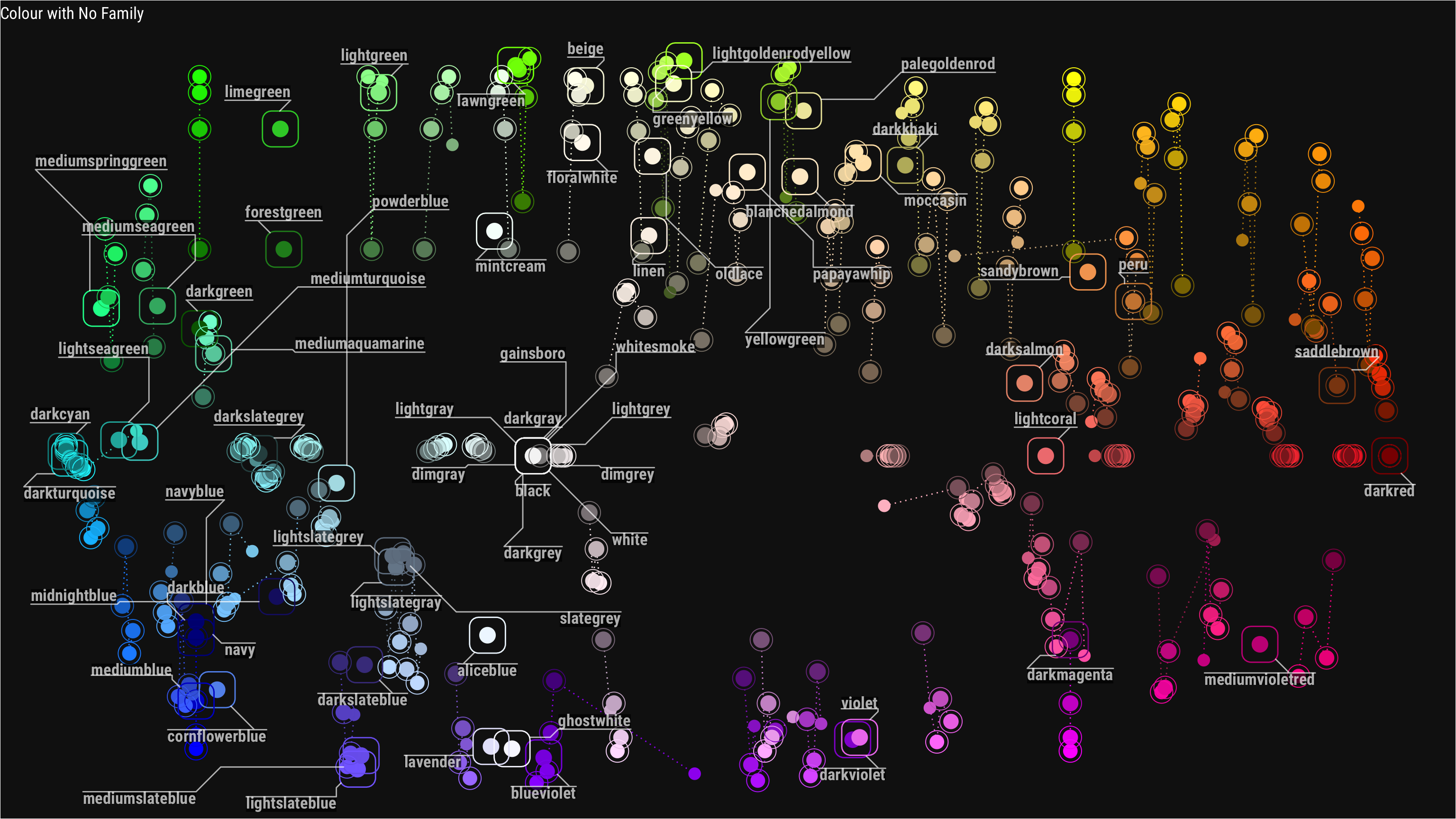
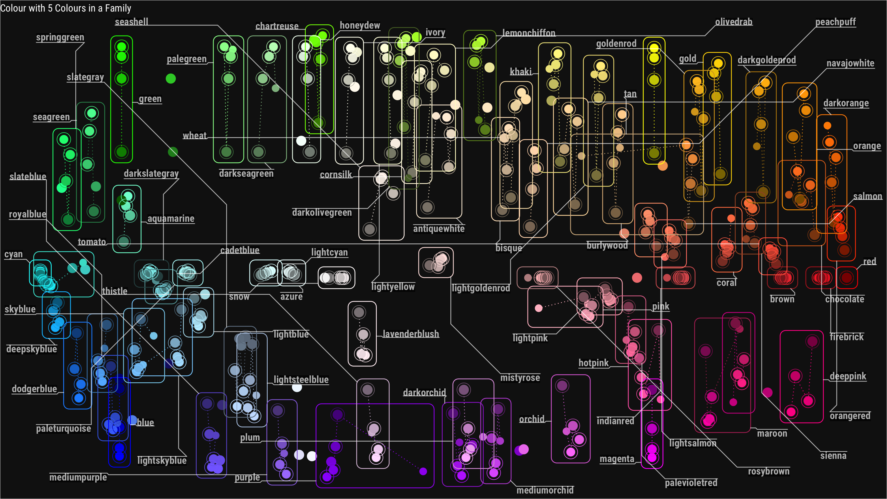
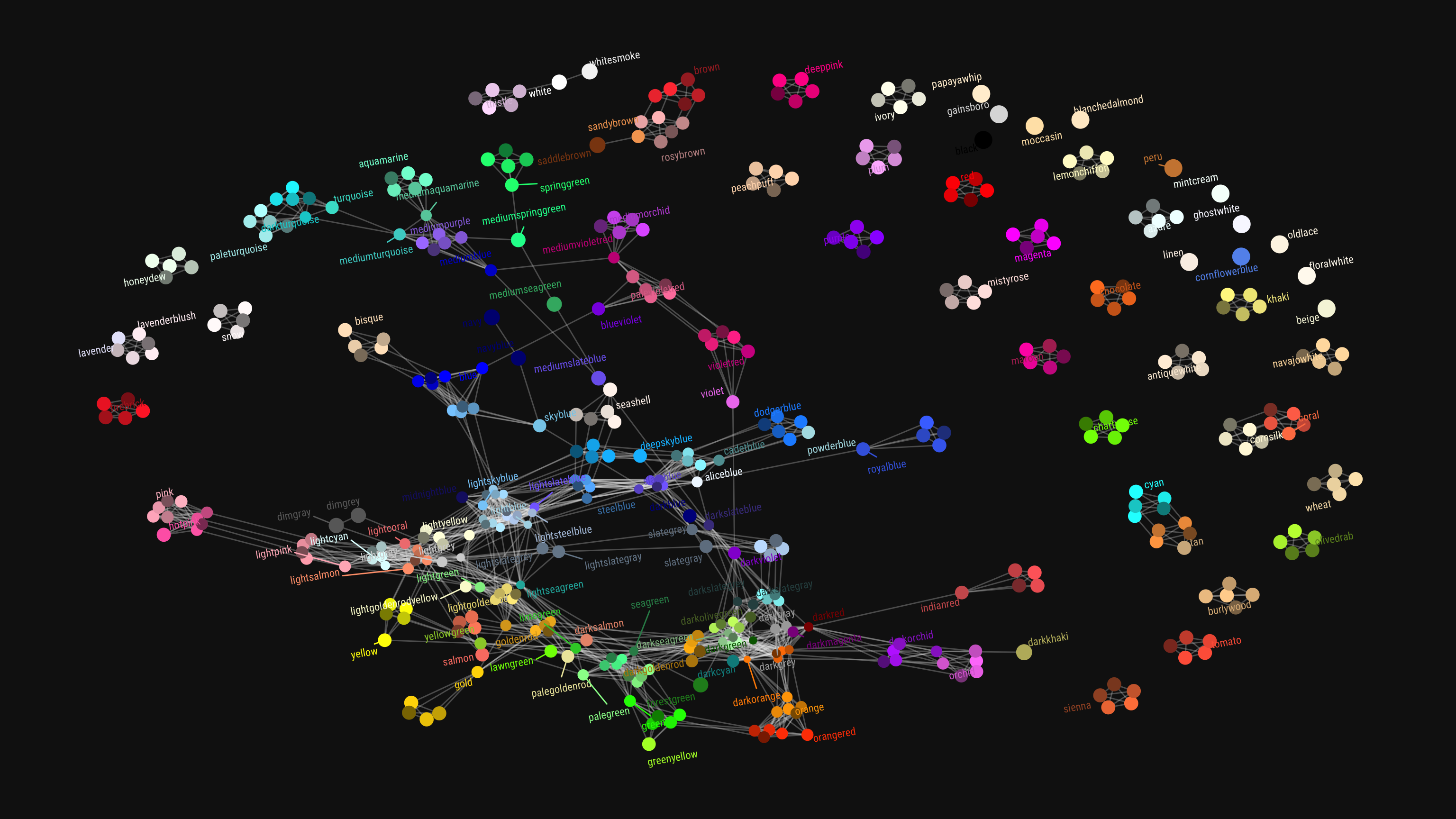
This last trick, I learned in this recent blog post I came across, by Chisato. She explored all colors() base R incorporates, using the new ggforce and ggraph packages (thank you Thomas Lin Petersen!). Her exploration resulted in some nice visual overviews, which you can view in more detail in the original blog here.
Colors() with no color familyColors() that have at least 5 colors in their familyColors() with similar names
Wanting to broaden your scope and learn a new programming language? This great workshop was given at EARL 2018 by Mango Solutions and helps R programmers transition into Python building on their existing R knowledge. The workshop includes exercises that introduce you to the key concepts of Python and some of its most powerful packages for data science, including numpy, pandas, sklearn, and seaborn.
Have a look at the associated workshop guide that walk you through the assignments, or at the github repo with all materials in Jupyter notebooks.


