Analytics in HR case study: Behind the scenes

Past week, Analytics in HR published a guest blog about one of my People Analytics projects which you can read here. In the blog, I explain why and how I examined the turnover of management trainees in light of the international work assignments they go on.

For the analyses, I used a statistical model called a survival analysis – also referred to as event history analysis, reliability analysis, duration analysis, time-to-event analysis, or proporational hazard models. It estimates the likelihood of an event occuring at time t, potentially as a function of certain data.

The sec version of surival analysis is a relatively easy model, requiring very little data. You can come a long way if you only have the time of observation (in this case tenure), and whether or not an event (turnover in this case) occured. For my own project, I had two organizations, so I added a source column as well (see below).

# LOAD REQUIRED PACKAGES ####
library(tidyverse)
library(ggfortify)
library(survival)

# SET PARAMETERS ####
set.seed(2)
sources = c("Organization Red","Organization Blue")
prob_leave = c(0.5, 0.5)
prob_stay = c(0.8, 0.2)
n = 60

# SIMULATE DATASETS ####
bind_rows(
  tibble(
    Tenure = sample(1:80, n*2, T),
    Source = sample(sources, n*2, T, prob_leave),
    Turnover = T
  ),
  tibble(
    Tenure = sample(1:85, n*25, T),
    Source = sample(sources, n*25, T, prob_stay),
    Turnover = F
  )
) ->
  data_surv

# RUN SURVIVAL MODEL ####
sfit <- survfit(Surv(data_surv$Tenure, event = data_surv$Turnover) ~ data_surv$Source)

# PLOT  SURVIVAL ####
autoplot(sfit, censor = F, surv.geom = 'line', surv.size = 1.5, conf.int.alpha = 0.2) +
  scale_x_continuous(breaks = seq(0, max(data_surv$Tenure), 12)) +
  coord_cartesian(xlim = c(0,72), ylim = c(0.4, 1)) +
  scale_color_manual(values = c("blue", "red")) +
  scale_fill_manual(values = c("blue", "red")) +
  theme_light() +
  theme(legend.background = element_rect(fill = "transparent"),
        legend.justification = c(0, 0),
        legend.position = c(0, 0),
        legend.text = element_text(size = 12)
        ) +
  labs(x = "Length of service", 
       y = "Percentage employed",
       title = "Survival model applied to the retention of new trainees",
       fill = "",
       color = "")

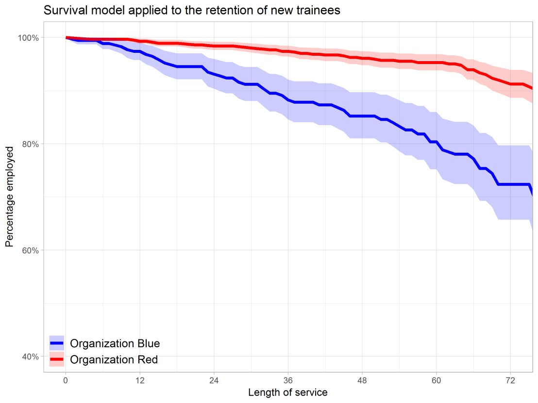
survival_plot — The resulting plot saved with ggsave, using width = 8 and height = 6.

Using the code above, you should be able to conduct a survival analysis and visualize the results for your own projects. Please do share your results!