It has been twenty years since the first Harry Potter novel, the sorcerer’s/philosopher’s stone, was published. To honour the series, I started a text analysis and visualization project, which my other-half wittily dubbed Harry Plotter. In several blogs, I intend to demonstrate how Hadley Wickham’s tidyverse and packages that build on its principles, such as tidytext (free book), have taken programming in R to an all-new level. Moreover, I just enjoy making pretty graphs : )

In this first blog (easier read), we will look at the sentiment throughout the books. In a second blog, we have examined the stereotypes behind the Hogwarts houses.
Setup
First, we need to set up our environment in RStudio. We will be needing several packages for our analyses. Most importantly, Bradley Boehmke was nice enough to gather all Harry Potter books in his harrypotter package on GitHub. We need devtools to install that package the first time, but from then on can load it in normally. Next, we load the tidytext package, which automates and tidies a lot of the text mining functionalities. We also need plyr for a specific function (ldply()). Other tidyverse packages we can load in a single bundle, including ggplot2, dplyr, and tidyr, which I use in almost every of my projects. Finally, we load the wordcloud visualization package which draws on tm.
After loading these packages, I set some additional default options.
library(harrypotter)
library(tidytext)
library(plyr)
library(tidyverse)
library(wordcloud)
options(stringsAsFactors = F,
scipen = 999,
max.print = 200)
theme_set(theme_light())
fs = 12
Data preparation
With RStudio set, its time to the text of each book from the harrypotter package which we then “pipe” (%>% – another magical function from the tidyverse – specifically magrittr) along to bind all objects into a single dataframe. Here, each row represents a book with the text for each chapter stored in a separate columns. We want tidy data, so we use tidyr’s gather() function to turn each column into grouped rows. With tidytext’s unnest_tokens() function we can separate the tokens (in this case, single words) from these chapters.
hp_words <- list(
philosophers_stone = philosophers_stone,
chamber_of_secrets = chamber_of_secrets,
prisoner_of_azkaban = prisoner_of_azkaban,
goblet_of_fire = goblet_of_fire,
order_of_the_phoenix = order_of_the_phoenix,
half_blood_prince = half_blood_prince,
deathly_hallows = deathly_hallows
) %>%
ldply(rbind) %>%
mutate(book = factor(seq_along(.id), labels = .id)) %>%
select(-.id) %>%
gather(key = 'chapter', value = 'text', -book) %>%
filter(!is.na(text)) %>%
mutate(chapter = as.integer(chapter)) %>%
unnest_tokens(word, text, token = 'words')
Let’s inspect our current data format with head(), which prints the first rows (default n = 6).
hp_words %>% head()
##                   book chapter  word
## 1   philosophers_stone       1   the
## 1.1 philosophers_stone       1   boy
## 1.2 philosophers_stone       1   who
## 1.3 philosophers_stone       1 lived
## 1.4 philosophers_stone       1    mr
## 1.5 philosophers_stone       1   and
Word frequency
A next step would be to examine word frequencies.
hp_words %>%
group_by(book, word) %>%
anti_join(stop_words, by = "word") %>%
count() %>%
arrange(desc(n)) %>%
group_by(book) %>%
mutate(top = seq_along(word)) %>%
filter(top <= 15) %>%
ggplot(aes(x = -top, fill = book)) +
geom_bar(aes(y = n), stat = 'identity', col = 'black') +
geom_text(aes(y = ifelse(n > max(n) / 2, max(n) / 50, n + max(n) / 50),
label = word), size = fs/3, hjust = "left") +
theme(legend.position = 'none',
text = element_text(size = fs),
axis.text.x = element_text(angle = 45, hjust = 1, size = fs/1.5),
axis.ticks.y = element_blank(),
axis.text.y = element_blank()) +
labs(y = "Word count", x = "",
title = "Harry Plotter: Most frequent words throughout the saga") +
facet_grid(. ~ book) +
coord_flip()
![]()

Unsuprisingly, Harry is the most common word in every single book and Ron and Hermione are also present. Dumbledore’s role as an (irresponsible) mentor becomes greater as the storyline progresses. The plot also nicely depicts other key characters:
- Lockhart and Dobby in book 2,
- Lupin in book 3,
- Moody and Crouch in book 4,
- Umbridge in book 5,
- Ginny in book 6,
- and the final confrontation with He who must not be named in book 7.
Finally, why does J.K. seem obsessively writing about eyes that look at doors?
Estimating sentiment
Next, we turn to the sentiment of the text. tidytext includes three famous sentiment dictionaries:
- AFINN: including bipolar sentiment scores ranging from -5 to 5
- bing: including bipolar sentiment scores
- nrc: including sentiment scores for many different emotions (e.g., anger, joy, and surprise)
The following script identifies all words that occur both in the books and the dictionaries and combines them into a long dataframe:
hp_senti <- bind_rows(
hp_words %>%
inner_join(get_sentiments("afinn"), by = "word") %>%
filter(score != 0) %>%
mutate(sentiment = ifelse(score < 0, 'negative', 'positive')) %>%
mutate(score = sqrt(score ^ 2)) %>%
group_by(book, chapter, sentiment) %>%
mutate(dictionary = 'afinn'),
hp_words %>%
inner_join(get_sentiments("bing"), by = "word") %>%
group_by(book, chapter, sentiment) %>%
mutate(dictionary = 'bing'),
hp_words %>%
inner_join(get_sentiments("nrc"), by = "word") %>%
group_by(book, chapter, sentiment) %>%
mutate(dictionary = 'nrc')
)
hp_senti %>% head()
## # A tibble: 6 x 6
## # Groups:   book, chapter, sentiment [2]
##                 book chapter      word score sentiment dictionary
##
## 1 philosophers_stone       1     proud     2  positive      afinn
## 2 philosophers_stone       1 perfectly     3  positive      afinn
## 3 philosophers_stone       1     thank     2  positive      afinn
## 4 philosophers_stone       1   strange     1  negative      afinn
## 5 philosophers_stone       1  nonsense     2  negative      afinn
## 6 philosophers_stone       1       big     1  positive      afinn
Wordcloud
Although wordclouds are not my favorite visualizations, they do allow for a quick display of frequencies among a large body of words.
hp_senti %>%
group_by(word) %>%
count() %>%
mutate(log_n = sqrt(n)) %>%
with(wordcloud(word, log_n, max.words = 100))
![]()

It appears we need to correct for some words that occur in the sentiment dictionaries but have a different meaning in J.K. Rowling’s books. Most importantly, we need to filter two character names.
hp_senti_sel <- hp_senti %>% filter(!word %in% c("harry","moody"))
Words per sentiment
Let’s quickly sketch the remaining words per sentiment.
hp_senti_sel %>%
group_by(word, sentiment) %>%
count() %>%
group_by(sentiment) %>%
arrange(sentiment, desc(n)) %>%
mutate(top = seq_along(word)) %>%
filter(top <= 15) %>%
ggplot(aes(x = -top, fill = factor(sentiment))) +
geom_bar(aes(y = n), stat = 'identity', col = 'black') +
geom_text(aes(y = ifelse(n > max(n) / 2, max(n) / 50, n + max(n) / 50),
label = word), size = fs/3, hjust = "left") +
theme(legend.position = 'none',
text = element_text(size = fs),
axis.text.x = element_text(angle = 45, hjust = 1),
axis.ticks.y = element_blank(),
axis.text.y = element_blank()) +
labs(y = "Word count", x = "",
title = "Harry Plotter: Words carrying sentiment as counted throughout the saga",
subtitle = "Using tidytext and the AFINN, bing, and nrc sentiment dictionaries") +
facet_grid(. ~ sentiment) +
coord_flip()
![]()

This seems ok. Let’s continue to plot the sentiment over time.
Positive and negative sentiment throughout the series
As positive and negative sentiment is included in each of the three dictionaries we can to compare and contrast scores.
plot_sentiment <- hp_senti_sel %>%
group_by(dictionary, sentiment, book, chapter) %>%
summarize(score = sum(score),
count = n(),
score = ifelse(is.na(score), count, score)) %>%
filter(sentiment %in% c('positive','negative')) %>%
mutate(score = ifelse(sentiment == 'negative', -score, score)) %>%
ggplot(aes(x = chapter, y = score)) +
geom_area(aes(fill = score > 0),stat = 'identity') +
scale_fill_manual(values = c('red','green')) +
geom_smooth(method = "loess", se = F, col = "black") +
theme(legend.position = 'none',
text = element_text(size = fs)) +
labs(x = "Chapter", y = "Sentiment score",
title = "Harry Plotter: Sentiment during the saga",
subtitle = "Using tidytext and the AFINN, bing, and nrc sentiment dictionaries") +
facet_grid(dictionary ~ book, scale = "free_x")
plot_sentiment
![]()

Let’s zoom in on the smoothed average.
plot_sentiment + coord_cartesian(ylim = c(-100,50))
![]()

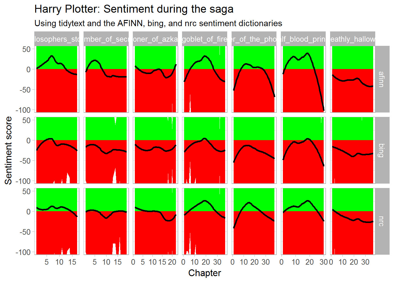
Sentiment seems overly negative throughout the series. Particularly salient is that every book ends on a down note, except the Prisoner of Azkaban. Moreover, sentiment becomes more volatile in books four through six. These start out negative, brighten up in the middle, just to end in misery again. In her final book, J.K. Rowling depicts a world about to be conquered by the Dark Lord and the average negative sentiment clearly resembles this grim outlook.
The bing sentiment dictionary estimates the most negative sentiment on average, but that might be due to this specific text.
Other emotions throughout the series
Finally, let’s look at the other emotions that are included in the nrc dictionary.
hp_senti_sel %>%
filter(!sentiment %in% c('negative','positive')) %>%
group_by(sentiment, book, chapter) %>%
count() %>%
ggplot(aes(x = chapter, y = n)) +
geom_area(aes(fill = sentiment), stat = 'identity') +
geom_smooth(aes(fill = sentiment), method = "loess", se = F, col = 'black') +
theme(legend.position = 'none',
text = element_text(size = fs)) +
labs(x = "Chapter", y = "Emotion score",
title = "Harry Plotter: Emotions during the saga",
subtitle = "Using tidytext and the nrc sentiment dictionary") +
facet_grid(sentiment ~ book, scale = "free_x")
![]()

This plot is less insightful as either the eight emotions are represented by similar words or J.K. Rowling combines all in her writing simultaneously. Patterns across emotions are highly similar, evidenced especially by the patterns in the Chamber of Secrets. In a next post, I will examine sentiment in a more detailed fashion, testing the differences over time and between characters statistically. For now, I hope you enjoyed these visualizations. Feel free to come back or subscribe to read my subsequent analyses.
The second blog in the Harry Plotter series examines the stereotypes behind the Hogwarts houses.


