Markdown is a great tool for integrating data analysis and report writing. Rosanna van Hespen wrote a great five-blog guide on how to write your thesis in R Markdown:

Disentangling Data Science
Tag: markdown
Markdown is a great tool for integrating data analysis and report writing. Rosanna van Hespen wrote a great five-blog guide on how to write your thesis in R Markdown:

Two weeks ago, I started the Harry Plotter project to celebrate the 20th anniversary of the first Harry Potter book. I could not have imagined that the first blog would be so well received. It reached over 4000 views in a matter of days thanks to the lovely people in the data science and #rstats community that were kind enough to share it (special thanks to MaraAverick and DataCamp). The response from the Harry Potter community, for instance on reddit, was also just overwhelming
All in all, I could not resist a sequel and in this second post we will explore the four houses of Hogwarts: Gryffindor, Hufflepuff, Ravenclaw, and Slytherin. At the end of today’s post we will end up with visualizations like this:

Various stereotypes exist regarding these houses and a textual analysis seemed a perfect way to uncover their origins. More specifically, we will try to identify which words are most unique, informative, important or otherwise characteristic for each house by means of ratio and tf-idf statistics. Additionally, we will try to estime a personality profile for each house using these characteristic words and the emotions they relate to. Again, we rely strongly on ggplot2 for our visualizations, but we will also be using the treemaps of treemapify. Moreover, I have a special surprise this second post, as I found the orginal Harry Potter font, which will definately make the visualizations feel more authentic. Of course, we will conduct all analyses in a tidy manner using tidytext and the tidyverse.
I hope you will enjoy this blog and that you’ll be back for more. To be the first to receive new content, please subscribe to my website www.paulvanderlaken.com, follow me on Twitter, or add me on LinkedIn. Additionally, if you would like to contribute to, collaborate on, or need assistance with a data science project or venture, please feel free to reach out.
All analysis were performed in RStudio, and knit using rmarkdown so that you can follow my steps.
In term of setup, we will be needing some of the same packages as last time. Bradley Boehmke gathered the text of the Harry Potter books in his harrypotter package. We need devtools to install that package the first time, but from then on can load it in as usual. We need plyr for ldply(). We load in most other tidyverse packages in a single bundle and add tidytext. Finally, I load the Harry Potter font and set some default plotting options.
# SETUP ####
# LOAD IN PACKAGES
# library(devtools)
# devtools::install_github("bradleyboehmke/harrypotter")
library(harrypotter)
library(plyr)
library(tidyverse)
library(tidytext)

# VIZUALIZATION SETTINGS
# custom Harry Potter font
# http://www.fontspace.com/category/harry%20potter
library(extrafont)
font_import(paste0(getwd(),"/fontomen_harry-potter"), prompt = F) # load in custom Harry Potter font
windowsFonts(HP = windowsFont("Harry Potter"))
theme_set(theme_light(base_family = "HP")) # set default ggplot theme to light
default_title = "Harry Plotter: References to the Hogwarts houses" # set default title
default_caption = "www.paulvanderlaken.com" # set default caption
dpi = 600 # set default dpiBefore we import and transform the data in one large piping chunk, I need to specify some variables.
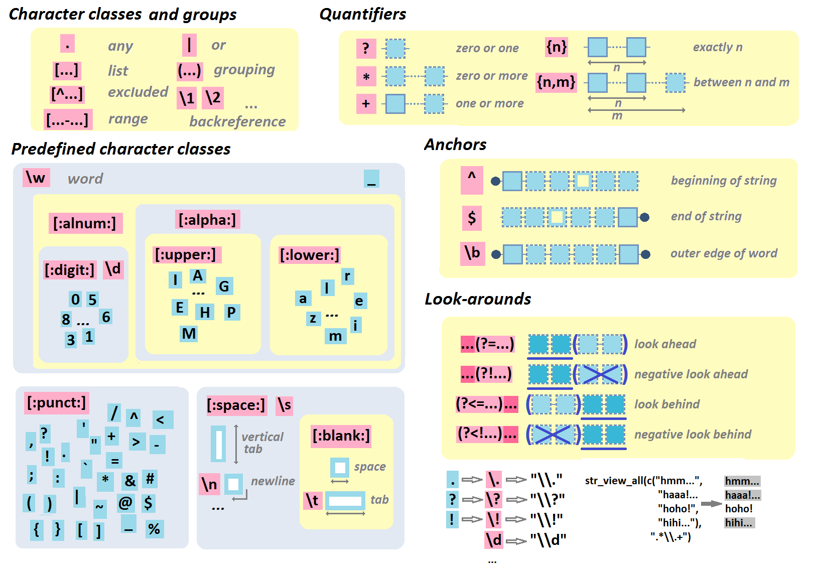
First, I tell R the house names, which we are likely to need often, so standardization will help prevent errors. Next, my girlfriend was kind enough to help me (colorblind) select the primary and secondary colors for the four houses. Here, the ggplot2 color guide in my R resources list helped a lot! Finally, I specify the regular expression (tutorials) which we will use a couple of times in order to identify whether text includes either of the four house names.
# DATA PREPARATION ####
houses <- c('gryffindor', 'ravenclaw', 'hufflepuff', 'slytherin') # define house names
houses_colors1 <- c("red3", "yellow2", "blue4", "#006400") # specify primary colors
houses_colors2 <- c("#FFD700", "black", "#B87333", "#BCC6CC") # specify secondary colors
regex_houses <- paste(houses, collapse = "|") # regular expressionOk, let’s import the data now. You may recognize pieces of the code below from last time, but this version runs slightly smoother after some optimalization. Have a look at the current data format.
# LOAD IN BOOK TEXT
houses_sentences <- list(
  `Philosophers Stone` = philosophers_stone,
  `Chamber of Secrets` = chamber_of_secrets,
  `Prisoner of Azkaban` = prisoner_of_azkaban,
  `Goblet of Fire` = goblet_of_fire,
  `Order of the Phoenix` = order_of_the_phoenix,
  `Half Blood Prince` = half_blood_prince,
  `Deathly Hallows` = deathly_hallows
) %>%
  # TRANSFORM TO TOKENIZED DATASET
  ldply(cbind) %>% # bind all chapters to dataframe
  mutate(.id = factor(.id, levels = unique(.id), ordered = T)) %>% # identify associated book
  unnest_tokens(sentence, `1`, token = 'sentences') %>% # seperate sentences
  filter(grepl(regex_houses, sentence)) %>% # exclude sentences without house reference
  cbind(sapply(houses, function(x) grepl(x, .$sentence)))# identify references
# examine
max.char = 30 # define max sentence length
houses_sentences %>%
  mutate(sentence = ifelse(nchar(sentence) > max.char, # cut off long sentences
                           paste0(substring(sentence, 1, max.char), "..."),
                           sentence)) %>%
  head(5)
## .id sentence gryffindor
## 1 Philosophers Stone "well, no one really knows unt... FALSE
## 2 Philosophers Stone "and what are slytherin and hu... FALSE
## 3 Philosophers Stone everyone says hufflepuff are a... FALSE
## 4 Philosophers Stone "better hufflepuff than slythe... FALSE
## 5 Philosophers Stone "there's not a single witch or... FALSE
## ravenclaw hufflepuff slytherin
## 1 FALSE TRUE TRUE
## 2 FALSE TRUE TRUE
## 3 FALSE TRUE FALSE
## 4 FALSE TRUE TRUE
## 5 FALSE FALSE TRUEOk, looking great, but not tidy yet. We need gather the columns and put them in a long dataframe. Thinking ahead, it would be nice to already capitalize the house names for which I wrote a custom Capitalize() function.
# custom capitalization function
Capitalize = function(text){
  paste0(substring(text,1,1) %>% toupper(),
         substring(text,2))
}

# TO LONG FORMAT
houses_long <- houses_sentences %>%
  gather(key = house, value = test, -sentence, -.id) %>%
  mutate(house = Capitalize(house)) %>% # capitalize names
  filter(test) %>% select(-test) # delete rows where house not referenced
# examine
houses_long %>%
  mutate(sentence = ifelse(nchar(sentence) > max.char, # cut off long sentences
                           paste0(substring(sentence, 1, max.char), "..."),
                           sentence)) %>%
  head(20)
## .id sentence house
## 1 Philosophers Stone i've been asking around, and i... Gryffindor
## 2 Philosophers Stone "gryffindor," said ron. Gryffindor
## 3 Philosophers Stone "the four houses are called gr... Gryffindor
## 4 Philosophers Stone you might belong in gryffindor... Gryffindor
## 5 Philosophers Stone " brocklehurst, mandy" went to... Gryffindor
## 6 Philosophers Stone "finnigan, seamus," the sandy-... Gryffindor
## 7 Philosophers Stone "gryffindor!" Gryffindor
## 8 Philosophers Stone when it finally shouted, "gryf... Gryffindor
## 9 Philosophers Stone well, if you're sure -- better... Gryffindor
## 10 Philosophers Stone he took off the hat and walked... Gryffindor
## 11 Philosophers Stone "thomas, dean," a black boy ev... Gryffindor
## 12 Philosophers Stone harry crossed his fingers unde... Gryffindor
## 13 Philosophers Stone resident ghost of gryffindor t... Gryffindor
## 14 Philosophers Stone looking pleased at the stunned... Gryffindor
## 15 Philosophers Stone gryffindors have never gone so... Gryffindor
## 16 Philosophers Stone the gryffindor first years fol... Gryffindor
## 17 Philosophers Stone they all scrambled through it ... Gryffindor
## 18 Philosophers Stone nearly headless nick was alway... Gryffindor
## 19 Philosophers Stone professor mcgonagall was head ... Gryffindor
## 20 Philosophers Stone over the noise, snape said, "a... GryffindorWoohoo, so tidy! Now comes the fun part: visualization. The following plots how often houses are mentioned overall, and in each book seperately.
# set plot width & height
w = 10; h = 6

# PLOT REFERENCE FREQUENCY
houses_long %>%
  group_by(house) %>%
  summarize(n = n()) %>% # count sentences per house
  ggplot(aes(x = desc(house), y = n)) +
  geom_bar(aes(fill = house), stat = 'identity') +
  geom_text(aes(y = n / 2, label = house, col = house),  # center text
            size = 8, family = 'HP') +
  scale_fill_manual(values = houses_colors1) +
  scale_color_manual(values = houses_colors2) +
  theme(axis.text.y = element_blank(),
        axis.ticks.y = element_blank(),
        legend.position = 'none') +
  labs(title = default_title,
       subtitle = "Combined references in all Harry Potter books",
       caption = default_caption,
       x = '', y = 'Name occurence') +
  coord_flip()
# PLOT REFERENCE FREQUENCY OVER TIME
houses_long %>%
  group_by(.id, house) %>%
  summarize(n = n()) %>% # count sentences per house per book
  ggplot(aes(x = .id, y = n, group = house)) +
  geom_line(aes(col = house), size = 2) +
  scale_color_manual(values = houses_colors1) +
  theme(legend.position = 'bottom',
        axis.text.x = element_text(angle = 15, hjust = 0.5, vjust = 0.5)) + # rotate x axis text
  labs(title = default_title,
       subtitle = "References throughout the Harry Potter books",
       caption = default_caption,
x = NULL, y = 'Name occurence', color = 'House') 
The Harry Potter font looks wonderful, right?
In terms of the data, Gryffindor and Slytherin definitely play a larger role in the Harry Potter stories. However, as the storyline progresses, Slytherin as a house seems to lose its importance. Their downward trend since the Chamber of Secrets results in Ravenclaw being mentioned more often in the final book (Edit – this is likely due to the diadem horcrux, as you will see later on).
I can’t but feel sorry for house Hufflepuff, which never really gets to involved throughout the saga.
Let’s dive into the specific words used in combination with each house. The following code retrieves and counts the single words used in the sentences where houses are mentioned.
# IDENTIFY WORDS USED IN COMBINATION WITH HOUSES
words_by_houses <- houses_long %>%
  unnest_tokens(word, sentence, token = 'words') %>% # retrieve words
  mutate(word = gsub("'s", "", word)) %>% # remove possesive determiners
  group_by(house, word) %>%
  summarize(word_n = n()) # count words per house
# examine
words_by_houses %>% head()
## # A tibble: 6 x 3
## # Groups: house [1]
## house word word_n
## <chr> <chr> <int>
## 1 Gryffindor 104 1
## 2 Gryffindor 22nd 1
## 3 Gryffindor a 251
## 4 Gryffindor abandoned 1
## 5 Gryffindor abandoning 1
## 6 Gryffindor abercrombie 1Now we can visualize which words relate to each of the houses. Because facet_wrap() has trouble reordering the axes (because words may related to multiple houses in different frequencies), I needed some custom functionality, which I happily recycled from dgrtwo’s github. With these reorder_within() and scale_x_reordered() we can now make an ordered barplot of the top-20 most frequent words per house.
# custom functions for reordering facet plots
# https://github.com/dgrtwo/drlib/blob/master/R/reorder_within.R
reorder_within <- function(x, by, within, fun = mean, sep = "___", ...) {
  new_x <- paste(x, within, sep = sep)
  reorder(new_x, by, FUN = fun)
}

scale_x_reordered <- function(..., sep = "___") {
  reg <- paste0(sep, ".+$")
  ggplot2::scale_x_discrete(labels = function(x) gsub(reg, "", x), ...)
}

# set plot width & height
w = 10; h = 7;

# PLOT MOST FREQUENT WORDS PER HOUSE
words_per_house = 20 # set number of top words
words_by_houses %>%
  group_by(house) %>%
  arrange(house, desc(word_n)) %>%
  mutate(top = row_number()) %>% # count word top position
  filter(top <= words_per_house) %>% # retain specified top number
  ggplot(aes(reorder_within(word, -top, house), # reorder by minus top number
             word_n, fill = house)) +
  geom_col(show.legend = F) +
  scale_x_reordered() + # rectify x axis labels
  scale_fill_manual(values = houses_colors1) +
  scale_color_manual(values = houses_colors2) +
  facet_wrap(~ house, scales = "free_y") + # facet wrap and free y axis
  coord_flip() +
  labs(title = default_title,
       subtitle = "Words most commonly used together with houses",
       caption = default_caption,
       x = NULL, y = 'Word Frequency')
Unsurprisingly, several stop words occur most frequently in the data. Intuitively, we would rerun the code but use dplyr::anti_join() on tidytext::stop_words to remove stop words.
# PLOT MOST FREQUENT WORDS PER HOUSE
# EXCLUDING STOPWORDS
words_by_houses %>%
  anti_join(stop_words, 'word') %>% # remove stop words
  group_by(house) %>%
  arrange(house, desc(word_n)) %>%
  mutate(top = row_number()) %>% # count word top position
  filter(top <= words_per_house) %>% # retain specified top number
  ggplot(aes(reorder_within(word, -top, house), # reorder by minus top number
             word_n, fill = house)) +
  geom_col(show.legend = F) +
  scale_x_reordered() + # rectify x axis labels
  scale_fill_manual(values = houses_colors1) +
  scale_color_manual(values = houses_colors2) +
  facet_wrap(~ house, scales = "free") + # facet wrap and free scales
  coord_flip() +
  labs(title = default_title,
       subtitle = "Words most commonly used together with houses, excluding stop words",
       caption = default_caption,
       x = NULL, y = 'Word Frequency')
However, some stop words have a different meaning in the Harry Potter universe. points are for instance quite informative to the Hogwarts houses but included in stop_words.
Moreover, many of the most frequent words above occur in relation to multiple or all houses. Take, for instance, Harry and Ron, which are in the top-10 of each house, or words like table, house, and professor.
We are more interested in words that describe one house, but not another. Similarly, we only want to exclude stop words which are really irrelevant. To this end, we compute a ratio-statistic below. This statistic displays how frequently a word occurs in combination with one house rather than with the others. However, we need to adjust this ratio for how often houses occur in the text as more text (and thus words) is used in reference to house Gryffindor than, for instance, Ravenclaw.
words_by_houses <- words_by_houses %>%
  group_by(word) %>% mutate(word_sum = sum(word_n)) %>% # counts words overall
  group_by(house) %>% mutate(house_n = n()) %>%
  ungroup() %>%
    # compute ratio of usage in combination with house as opposed to overall
  # adjusted for house references frequency as opposed to overall frequency
  mutate(ratio = (word_n / (word_sum - word_n + 1) / (house_n / n())))
# examine
words_by_houses %>% select(-word_sum, -house_n) %>% arrange(desc(word_n)) %>% head()
## # A tibble: 6 x 4
## house word word_n ratio
## <chr> <chr> <int> <dbl>
## 1 Gryffindor the 1057 2.373115
## 2 Slytherin the 675 1.467926
## 3 Gryffindor gryffindor 602 13.076218
## 4 Gryffindor and 477 2.197259
## 5 Gryffindor to 428 2.830435
## 6 Gryffindor of 362 2.213186# PLOT MOST UNIQUE WORDS PER HOUSE BY RATIO
words_by_houses %>%
group_by(house) %>%
arrange(house, desc(ratio)) %>%
mutate(top = row_number()) %>% # count word top position
filter(top <= words_per_house) %>% # retain specified top number
ggplot(aes(reorder_within(word, -top, house), # reorder by minus top number
ratio, fill = house)) +
geom_col(show.legend = F) +
scale_x_reordered() + # rectify x axis labels
scale_fill_manual(values = houses_colors1) +
scale_color_manual(values = houses_colors2) +
facet_wrap(~ house, scales = "free") + # facet wrap and free scales
coord_flip() +
labs(title = default_title,
subtitle = "Most informative words per house, by ratio",
caption = default_caption,
x = NULL, y = 'Adjusted Frequency Ratio (house vs. non-house)')
# PS. normally I would make a custom ggplot function
#    when I plot three highly similar graphs
This ratio statistic (x-axis) should be interpreted as follows: night is used 29 times more often in combination with Gryffindor than with the other houses.
Do you think the results make sense:
Honestly, I was not expecting such good results! However, there is always room for improvement.
We may want to exclude words that only occur once or twice in the book (e.g., Alecto) as well as the house names. Additionally, these barplots are not the optimal visualization if we would like to include more words per house. Fortunately, Hadley Wickham helped me discover treeplots. Let’s draw one using the ggfittext and the treemapify packages.
# set plot width & height
w = 12; h = 8;

# PACKAGES FOR TREEMAP
# devtools::install_github("wilkox/ggfittext")
# devtools::install_github("wilkox/treemapify")
library(ggfittext)
library(treemapify)


# PLOT MOST UNIQUE WORDS PER HOUSE BY RATIO
words_by_houses %>%
  filter(word_n > 3) %>% # filter words with few occurances
  filter(!grepl(regex_houses, word)) %>% # exclude house names
  group_by(house) %>%
  arrange(house, desc(ratio), desc(word_n)) %>%
  mutate(top = seq_along(ratio)) %>%
  filter(top <= words_per_house) %>% # filter top n words
  ggplot(aes(area = ratio, label = word, subgroup = house, fill = house)) +
  geom_treemap() + # create treemap
  geom_treemap_text(aes(col = house), family = "HP", place = 'center') + # add text
  geom_treemap_subgroup_text(aes(col = house), # add house names
                             family = "HP", place = 'center', alpha = 0.3, grow = T) +
  geom_treemap_subgroup_border(colour = 'black') +
  scale_fill_manual(values = houses_colors1) +
  scale_color_manual(values = houses_colors2) +
  theme(legend.position = 'none') +
  labs(title = default_title,
       subtitle = "Most informative words per house, by ratio",
       caption = default_caption)
A treemap can display more words for each of the houses and displays their relative proportions better. New words regarding the houses include the following, but do you see any others?
In the earlier code, we specified a minimum number of occurances for words to be included, which is a bit hacky but necessary to make the ratio statistic work as intended. Foruntately, there are other ways to estimate how unique or informative words are to houses that do not require such hacks.
tf-idf similarly estimates how unique / informative words are for a body of text (for more info: Wikipedia). We can calculate a tf-idf score for each word within each document (in our case house texts) by taking the product of two statistics:
A high tf-idf score means that a word occurs relatively often in a specific document and not often in other documents. Different weighting schemes can be used to td-idf’s performance in different settings but we used the simple default of tidytext::bind_tf_idf().
An advantage of tf-idf over the earlier ratio statistic is that we no longer need to specify a minimum frequency: low frequency words will have low tf and thus low tf-idf. A disadvantage is that tf-idf will automatically disregard words occur together with each house, be it only once: these words have zero idf (log(4/4)) so zero tf-idf.
Let’s run the treemap gain, but not on the computed tf-idf scores.
words_by_houses <- words_by_houses %>%
  # compute term frequency and inverse document frequency
  bind_tf_idf(word, house, word_n)
# examine
words_by_houses %>% select(-house_n) %>% head()
## # A tibble: 6 x 8
## house word word_n word_sum ratio tf idf
## <chr> <chr> <int> <int> <dbl> <dbl> <dbl>
## 1 Gryffindor 104 1 1 2.671719 6.488872e-05 1.3862944
## 2 Gryffindor 22nd 1 1 2.671719 6.488872e-05 1.3862944
## 3 Gryffindor a 251 628 1.774078 1.628707e-02 0.0000000
## 4 Gryffindor abandoned 1 1 2.671719 6.488872e-05 1.3862944
## 5 Gryffindor abandoning 1 2 1.335860 6.488872e-05 0.6931472
## 6 Gryffindor abercrombie 1 1 2.671719 6.488872e-05 1.3862944
## # ... with 1 more variables: tf_idf <dbl># PLOT MOST UNIQUE WORDS PER HOUSE BY TF_IDF
words_per_house = 30
words_by_houses %>%
filter(tf_idf > 0) %>% # filter for zero tf_idf
group_by(house) %>%
arrange(house, desc(tf_idf), desc(word_n)) %>%
mutate(top = seq_along(tf_idf)) %>%
filter(top <= words_per_house) %>%
ggplot(aes(area = tf_idf, label = word, subgroup = house, fill = house)) +
geom_treemap() + # create treemap
geom_treemap_text(aes(col = house), family = "HP", place = 'center') + # add text
geom_treemap_subgroup_text(aes(col = house), # add house names
family = "HP", place = 'center', alpha = 0.3, grow = T) +
geom_treemap_subgroup_border(colour = 'black') +
scale_fill_manual(values = houses_colors1) +
scale_color_manual(values = houses_colors2) +
theme(legend.position = 'none') +
labs(title = default_title,
subtitle = "Most informative words per house, by tf-idf",
caption = default_caption)
This plot looks quite different from its predecessor. For instance, Marcus Flint and Adrian Pucey are added to house Slytherin and Hufflepuff’s main color is indeed not just yellow, but canary yellow. Severus Snape’s dual role is also nicely depicted now, with him in both house Slytherin and house Gryffindor. Do you notice any other important differences? Did we lose any important words because they occured in each of our four documents?
We end this second Harry Plotter blog by examining to what the extent the stereotypes that exist of the Hogwarts Houses can be traced back to the books. To this end, we use the NRC sentiment dictionary, see also the the previous blog, with which we can estimate to what extent the most informative words for houses (we have over a thousand for each house) relate to emotions such as anger, fear, or trust.
The code below retains only the emotion words in our words_by_houses dataset and multiplies their tf-idf scores by their relative frequency, so that we retrieve one score per house per sentiment.
# PLOT SENTIMENT OF INFORMATIVE WORDS (TFIDF)
words_by_houses %>%
  inner_join(get_sentiments("nrc"), by = 'word') %>%
  group_by(house, sentiment) %>%
  summarize(score = sum(word_n / house_n * tf_idf)) %>% # compute emotion score
  ggplot(aes(x = house, y = score, group = house)) +
  geom_col(aes(fill = house)) + # create barplots
  geom_text(aes(y = score / 2, label = substring(house, 1, 1), col = house),
            family = "HP", vjust = 0.5) + # add house letter in middle
  facet_wrap(~ Capitalize(sentiment), scales = 'free_y') + # facet and free y axis
  scale_fill_manual(values = houses_colors1) +
  scale_color_manual(values = houses_colors2) +
  theme(legend.position = 'none', # tidy dataviz
        axis.text.y = element_blank(),
        axis.ticks.y = element_blank(),
        axis.text.x = element_blank(),
        axis.ticks.x = element_blank(),
        strip.text.x = element_text(colour = 'black', size = 12)) +
  labs(title = default_title,
       subtitle = "Sentiment (nrc) related to houses' informative words (tf-idf)",
       caption = default_caption,
       y = "Sentiment score", x = NULL)
The results to a large extent confirm the stereotypes that exist regarding the Hogwarts houses:
With this we have come to the end of the second part of the Harry Plotter project, in which we used tf-idf and ratio statistics to examine which words were most informative / unique to each of the houses of Hogwarts. The data was retrieved using the harrypotter package and transformed using tidytext and the tidyverse. Visualizations were made with ggplot2 and treemapify, using a Harry Potter font.
I have several ideas for subsequent posts and I’d love to hear your preferences or suggestions:
For now, I hope you enjoyed this blog and that you’ll be back for more. To receive new content first, please subscribe to my website www.paulvanderlaken.com, follow me on Twitter, or add me on LinkedIn.
If you would like to contribute to, collaborate on, or need assistance with a data science project or venture, please feel free to reach out
Help yourself to these free books, tutorials, packages, cheat sheets, and many more materials for R programming. There’s a separate overview for handy R programming tricks. If you have additions, please comment below or contact me!
LAST UPDATED: 2021-09-24
Completely new to R? → Start learning here!
swirl()***tidyverseroxygen2 by Hadley Wickhamknitr by Yihui Xieknitr in a nutshell: a minimal tutorial by Karl Bromandevtools – tools to make an R developer’s life easier roxygen2 – tools for describing functions in comments next to their definitions Rd2roxygen – tools for converting Rd to roxygen documentationtestthat – tools that simplify the testing of R packagestidyeval tutorial by Ian Lyttle purrr tutorial by Jenny Bryan***purrr tutorial by Emorie Beckpurrr tutorial by Dan Ovandopurrr cheat sheet by RStudiodata.table cheat sheet by Erik Petrovskidata.table wide cheat sheet by DataCampdata.table long cheat sheet by DataCamptidyverse cheat sheet by DataCampreadr, tibble, and tidyrforcats cheat sheet by Lise Vaudordplyrdplyr and sjmiscggplot2dplyr and tidyrrandomizr by Alex Coppock.mosaic package teaching math, stats, computation, and modelling, by Michael Laviolettestringrlubridatepurrr functional programming cheat sheet by RStudiocartography cheat sheet by Timothee Giraudbayesplot cheat sheet by Edward Roualdesdevtoolsxts cheat sheet for time series by DataCampreticulate cheat sheet by RStudioMany of the above cheat sheets are hosted in the official RStudio cheat sheet overview.
data.tabledata.table & dplyr codedata.table cheat sheet by Erik Petrovskidata.table wide cheat sheet by DataCampdata.table long cheat sheet by DataCamp dplyr cheat sheet by RStudiocolourpicker – widget that allows users to choose colourspaletteer – comprehensive collection of color palettes in R***ggthemes::scale_color_canvaplotly – interactive plotsbillboarder – easy interface to billboard.js, a JavaScript chart library based on D3d3heatmap – interactive D3 heatmapsaltair – Vega-Lite visualizations via PythonDT – interactive tablesDiagrammeR – interactive diagrams (DiagrammeR cheat sheet)dygraphs – interactive time series plotsformattable – formattable data structuresggvis – interactive ggplot2highcharter – interactive Highcharts plotsleaflet – interactive mapsmetricsgraphics – interactive JavaScript bare-bones line, scatterplot and bar chartsnetworkD3 – interative D3 network graphsscatterD3 – interactive scatterplots with D3rbokeh – interactive Bokeh plotsrCharts – interactive Javascript chartsrcdimple – interactive JavaScript bar charts and othersrglwidget – interactive 3d plotsthreejs – interactive 3d plots and globesvisNetwork – interactive network graphswordcloud2 – interface to wordcloud2.js.timevis – interactive timelinesggplot2ggthemrpatchwork or cowplotequisse – RStudio addin to interactively explore data with ggplot2 without codingggthemes – plot style themeshrbrthemes – opinionated, typographic-centric themesggmap – maps with Google Maps, Open Street Maps, etc.ggiraph – interactive ggplotsgghighight – highlight lines or values, see vignetteggstance – horizontal versions of common plotsGGally – scatterplot matricesggalt – additional coordinate systems, geoms, etc.ggbeeswarm – column scatter plots or voilin scatter plotsggforce – additional geoms, see visual guideggrepel – prevent plot labels from overlappingggraph – graphs, networks, trees and moreggpmisc – photo-biology related extensionsgeomnet – network visualizationggExtra – marginal histograms for a plotgganimate – animations, see also the gganimate wiki pageggpage – pagestyled visualizations of text based dataggpmisc – useful additional geom_* and stat_* functionsggstatsplot – include details from statistical tests in plotsggspectra – tools for plotting light spectraggnetwork – geoms to plot networksggpoindensity – cross between a scatter plot and a 2D density plotggradar – radar chartsggsurvplot (survminer) – survival curvesggseas – seasonal adjustment toolsggthreed – (evil) 3D geomsggtech – style themes for plotsggtern – ternary diagramsggTimeSeries – time series visualizationsggtree – tree visualizationstreemapify – wilcox’s treemapsseewave – spectograms coefplot – visualizes model statisticscirclize – circular visualizations for categorical dataclustree – visualize clustering analysisquantmod – candlestick financial chartsdabestr– Data Analysis using Bootstrap-Coupled ESTimationdevoutsvg – an SVG graphics device (with pattern fills)devoutpdf – an PDF graphics device cartography – create and integrate maps in your R workflowcolorspace – HSL based color palettesviridis – Matplotlib viridis color pallete for Rmunsell – Munsell color palettes for RCairo – high-quality display outputigraph – Network Analysis and Visualizationgraphlayouts – new layout algorithms for network visualization lattice – Trellis graphicstmap – thematic mapstrelliscopejs – interactive alternative for facet_wraprgl – interactive 3D plotscorrplot – graphical display of a correlation matrixgoogleVis – Google Charts APIplotROC – interactive ROC plotsextrafont – fonts in R graphicsrvg – produces Vector Graphics that allow further editing in PowerPoint or Excelshowtext – text using system fontsanimation – animated graphics using ImageMagick.misc3d – 3d plots, isosurfaces, etc.xkcd – xkcd style graphicsimager – CImg library to work with imagesungeviz – tools for visualize uncertaintywaffle – square pie charts a.k.a. waffle chartshht, warbleR, soundgen, signal, seewave, or phonToolsflexdashboard – dashboard creation simplifiedcolourpicker – widget that allows users to choose coloursbrighter – toolbox with helpful functions for shiny developmentDesktopDeployR – self-contained R-based desktop applicationsknitr book (Xie, 2015)xaringan by Yihui Xiexariganblogdown websites with R Markdown (Xie, Thomas, & Hill, 2018)blogdown tutorialsblogdown in R, by Storybenchtidystats – automating updating of model statisticspapaja – preparing APA journal articlesblogdown – build websites with Markdown & Hugohuxtable – create Excel, html, & LaTeX tablesxaringan – make slideshows via remark.js and markdown summarytools – produces neat, quick data summary tables citr – RStudio Addin to Insert Markdown Citations googlesheetssparklyr by DataCampRMySQL – connects to MySQL and MariaDBRPostgreSQL – connects to Postgres and Redshift.RSQLite – embeds a SQLite database.odbc – connects to many commercial databases via the open database connectivity protocol.bigrquery – connects to Google’s BigQuery.DBI – separates the connectivity to the DBMS into a “front-end” and a “back-end”.dbplot – leverages dplyr to process calculations of plot inside databasedplyr – also works with remote on-disk data stored in databasestidypredict – run predictions inside the databasecaretmlr cheat sheet by Aaron Coleykeras cheat sheet by RStudiocaret cheat sheet by Max Kuhnnardl cheat sheet by Taha Zaghdoudisurvminer cheat sheet by Przemysław Bieceksparklyr cheat sheet by RStudioxts cheat sheettsfeatures packagetidyquantxts – extensible time seriestsfeatures – methods for extracting various features from time series data tidyquant – tidyverse-style financial analysis survival – functionality for survival and hazard modelsggsurvplot (survminer) – survival curvescorrr – easier correlation matrix management and explorationtmtidytextrtweettwitteRquanteda cheat sheet by Stefan Müller and Kenneth Benoittm – text mining.tidytext – text mining using tidyverse principlesquanteda – framework for quantitative text analysisgutenbergr – public domain works (free books to practice on)corpora – statistics and data sets for corpus frequency data.tau – Text Analysis UtilitiesSentiment140 – headache-free sentiment analysissentimentr – sentiment analysis using text polarityopenNLP – sentence detector, tokenizer, pos-tagger, shallow and full syntactic parser, named-entity detector, and maximum entropy models with OpenNLP.cleanNLP – natural language processing via tidy data modelsRSentiment – English lexicon-based sentiment analysis with negation and sarcasm detection functionalities.RWeka – data mining tasks with Wekawordnet – a large lexical database of English with WordNet .stringi – language processing wrapperstextcat – provides support for n-gram based text categorization.text2vec – text vectorization, topic modeling (LDA, LSA), word embeddings (GloVe), and similarities.lsa – Latent Semantic Analysistopicmodels -Latent Dirichlet Allocation (LDA) and Correlated Topics Models (CTM)lda -Latent Dirichlet Allocation and related modelsregexplain – interactive RStudio addin for regular expressionssf) cheat sheet by Ryan GarnettDescriptions mostly taken from their own websites:
jmv – free and open statistical software to bridge the gap between researcher and statisticianreadxl – package to load in Excel dataxlsx – package to read and write Excel datarvg – produces Vector Graphics which can be modified in Exceldevoutpdf – an PDF graphics device tidyxl – imports non-tabular (e.g., format) data from Excel files into Runpivotr – unpivot complex and irregular data layouts in Runheadr – handle data with embedded subheadersreticulate cheat sheet by RStudio reticulate – tools for interoperability between Python and Rsqldf – running SQL statements on R data frames