Apparently, I was not the only geek who decided to celebrate the 20th anniversary of the Harry Potter saga with statistical analysis. Students Moritz Haine and Markus Dienstknecht of the Data Science for Decision Making Master at Maastricht University started their own celebratory project as part of a course Information Retrieval and Text Mining.
Students in previous years looked at for example Lord of the Rings, Star Wars and Game of Thrones. However, to our surprise, Harry Potter was missing. Since the books are about magic, we decided it would be interesting to identify all of the spells and the wizards that cast the most spells
Moritz Haine
From the books, the students extracted 41 different wizards, 64 different spells and 253 spells. Moritz points out that they could only include spoken spells, even though the most powerful wizards can also cast spells without naming them. They expect this might be the reason why Dumbledore and Voldemort are not ranked as high. At the end of their project, Moritz and Markus visualized their results in a spell-character mapping.
A network mapping of the characters and spells casted in the Harry Potter saga [original]This is the latest addition to my collection of Harry Potter analyses, to which a similar, interactive web application of spell usage was added only last week.
The following is the first part of my introduction to regular expression (regex), in general, and the use of regex in R, in specific. It is loosely inspired on the swirl() tutorial by Jon Calder. I created it in R Markdown and uploaded it to RPubs, for an easier read.
Regular expression
A regular expression, regex or regexp (sometimes called a rational expression) is, in theoretical computer science and formal language theory, a sequence of characters that define a search pattern. Usually this pattern is then used by string searching algorithms for “find” or “find and replace” operations on strings (Wikipedia). Regular expressions were originally developed for the Perl language and have since been implemented in many other languages including R.
Regular expressions usually involve two parts: a pattern and a text string. The pattern defines what type and/or sequence of characters to look for whereas the text string represents the content in which to search/match this pattern. Patterns are always strings themselves and thus need to be enclosed in (single or double) quotation marks.
Example
An example: the pattern “stat” will match the occurance of the letters “s”, “t”, “a”, “t” in that specific order. Regardless of where in the content (text string) they occur and what other characters may precede the “s” or follow the last “t”.
Base R’s grepl() function returns a logical value reflecting whether the pattern is matched. The below demonstrates how the pattern “stats” can be found in both “statistics” and “estate” but not in “castrate” (which does include the letters, but with an r in between), in “catalyst” (which does include the letters, but not in the right order), or in “banana” (which does not include all the letters).
Moreover, regular expressions are case sensitive, so “stat” is not found in “Statistics”, unless it is specified that case should be ignored (FALSE by default).
Base R includes seven main functions that use regular expressions with different outcomes. These are grep(), grepl(), regexpr(), gregexpr(), regexec(), sub(), and gsub(). Although they require mostly similar inputs, their returned values are quite different.
grep() & grepl()
grep() examines each element of a character vector and returns the indices where the pattern is matched.
sentences=c("I like statistics", "I like bananas", "Estates and statues are expensive")grep("stat", sentences)
## [1] 1 3
By setting the value parameter to TRUE, grep() will return the character element instead of its index.
grep("stat", sentences, value=TRUE)
## [1] "I like statistics" "Estates and statues are expensive"
It’s logical brother grepl() you’ve seen before. It returns a logical value instead of the index or the element.
grepl("stat", sentences)
## [1] TRUE FALSE TRUE
regexpr() & gregexpr()
regexpr() seeks for a pattern in a text and returns an integer vector with two attributes (also vectors). The main integer vector returned represents the position where the pattern was first matched in the text. Its attribute “match.length” is also an integer vector representing the length of the match (in this case “stat” is always length 4).
If the pattern is not matched, both of the main vector and the length attribute will have a value of -1.
The second attribute (“useBytes”) is always a logical vector of length one. It represents whether matching is done byte-by-byte (TRUE) or character-by-character (FALSE), but you may disregard it for now.
sentences
## [1] "I like statistics"                 "I like bananas"
## [3] "Estates and statues are expensive"
Note that, for the third sentence, regexpr() only returns the values for the first match (i.e., “Estate”) but not those of the second match (i.e., “statues”). For this reason, the function has a brother, gregexpr(), which has the same functionality but performs the matching on a global scale (hence the leading g). This means that the algorithm does not stop after its first match, but continues and reports all matches within the content string.
grepexpr() thus does not return a single vector, but a list of vectors. Each of these vectors reflects an input content string as is the length of the number of matches within that content. For example, the “stat” pattern is matched twice in our third sentence, therefore its vector is length 2, with the starting position of each match as well as their lengths.
sentences
## [1] "I like statistics"                 "I like bananas"
## [3] "Estates and statues are expensive"
In order to explain how regexec() differs from gregexpr(), we first need to explain how parentheses in work in regex. Most simply speaking, parentheses or round brackets (()) indicate groups. One of the advantages of groups is that logical tests can thus be conducted within regular expressions.
sentences
## [1] "I like statistics"                 "I like bananas"
## [3] "Estates and statues are expensive"
grepl("like", sentences)
## [1] TRUE TRUE FALSE
grepl("are", sentences)
## [1] FALSE FALSE TRUE
grepl("(are|like)", sentences)
## [1] TRUE TRUE TRUE
regexec()
However, these groups can also be useful to extract more detailed information from a regular expression. This is where regexec() comes in.
Like gregexpr(), regexec() returns a list of the same length as the content. This list includes vectors that reflect the starting positions of the overall match, as well as the matches corresponding to parenthesized subpatterns. Similarly, attribute “match.length” reflects the lengths of each of the overall and submatches. In case no match is found, a -1 value is again returned.
The beauty of regexec() because clear when we split our pattern into two groups using parentheses: “(st)(at)”. As you can see below, both regexpr() and its global brother gregexpr() disregard this grouping and provide the same output as before – as you would expect for the pattern “stat”. In contast, regexec() notes that we now have a global pattern (“stat”)as well as two subpatterns (“st” and “at”). For each of these, the function returns the starting positions as well as the pattern lengths.
sentences
## [1] "I like statistics"                 "I like bananas"
## [3] "Estates and statues are expensive"
The final two base regex functions are sub() and its global brother gsub(). These, very intiutively, substitute a matched pattern by a specified replacement and then return all inputs. For instance, we could replace “I” with “You” in our example sentences.
sub(pattern="I", replacement="You", sentences)
## [1] "You like statistics"               "You like bananas"
## [3] "Estates and statues are expensive"
Similarly, we could desire to replace all spaces by underscores. This would require a global search (i.e., gsub()), as sub() would stop after the first match.
This was the first part of my introduction to Regular Expression in R. For more information detailed information about all input parameters of each function, please consult the base R manual. In subsequent parts, I will introduce you to so-called Anchors, Character Classes, Groups, Ranges, and Quantifiers. These will allow you to perform more advanced searches and matches. Here, we will also elaborate on lazy, greedy, and possesive regular expressions, which further expand our search capability as well as flexibility.
In the end, I hope to provide you with an overview of several Regular Expressions that I have found extremely useful in my personal project, and which should be valuable to anyone who conducts applied research (in organizations).
This blog summarized work that has been posted here, here, and here.
Iain of degeneratestate.org wrote a three-piece series where he applied text mining to the lyrics of 222,623 songs from 7,364 heavy metal bands spread over 22,314 albums that he scraped from darklyrics.com. He applied a broad range of different analyses in Python, the code of which you can find here on Github.
For example, he starts part 1 by calculated the difficulty/complexity of the lyrics of each band using the Simple Measure of Gobbledygook or SMOG and contrasted this to the number of swearwords used, finding a nice correlation.
Lyric complexity relates positive to swearwords used.
Furthermore, he ran some word importance analysis, looking at word frequencies, log-likelihood ratios, and TF-IDF scores. This allowed him to contrast the word usage of the different bands, finding, for instance, one heavy metal band that was characterized by the words “oh yeah baby got love“: fans might recognize either Motorhead, Machinehead, or Diamondhead.
Using cosine distance measures, Iain could compare the word vectors of the different bands, ultimately recognizing band similarity, and song representativeness for a band. This allowed interesting analysis, such as a clustering of the various bands:
However, all his analysis worked out nicely. While he also applied t-SNE to visualize band similarity in a two-dimensional space, the solution was uninformative due to low variance in the data.
He could predict the band behind a song by training a one-vs-rest logistic regression classifier based on the reduced lyric space of 150 dimensions after latent semantic analysis. Despite classifying a song to one of 120 different bands, the classifier had a precision and recall both around 0.3, with negligible hyper parameter tuning. He used the classification errors to examine which bands get confused with each other, and visualized this using two network graphs.
His first approach was to use probabilistic distributions known as language models. Basically he develops a Markov Chain, in his opinion more of a “unsmoothed maximum-likelihood language model“, which determines the next most probable word based on the previous word(s). This model is based on observed word chains, for instance, those in the first two lines to Iron Maiden’s Number of the Beast:
Another approach would be to train a neural network. Iain used Keras, which ran on an amazon GPU instance. He recognizes the power of neural nets, but says they also come at a cost:
“The maximum likelihood models we saw before took twenty minutes to code from scratch. Even using powerful libraries, it took me a while to understand NNs well enough to use. On top of this, training the models here took days of computer time, plus more of my human time tweeking hyper parameters to get the models to converge. I lack the temporal, financial and computational resources to fully explore the hyperparameter space of these models, so the results presented here should be considered suboptimal.” – Iain
He started out with feed forward networks on a character level. His best try consisted of two feed forward layers of 512 units, followed by a softmax output, with layer normalisation, dropout and tanh activations, which he trained for 20 epochs to minimise the mean cross-entropy. Although it quickly beat the maximum likelihood Markov model, its longer outputs did not look like genuine heavy metal songs.
So he turned to recurrent neural network (RNN). The RNN Iain used contains two LSTM layers of 512 units each, followed by a fully connected softmax layer. He unrolled the sequence for 32 characters and trained the model by predicting the next 32 characters, given their immediately preceding characters, while minimizing the mean cross-entropy:
“To generate text from the RNN model, we step character-by-character through a sequence. At each step, we feed the current symbol into the model, and the model returns a probability distribution over the next character. We then sample from this distribution to get the next character in the sequence and this character goes on to become the next input to the model. The first character fed into the model at the beginning of generation is always a special start-of-sequence character.” – Iain
This approach worked quite well, and you can compare and contrast it with the earlier models here. If you’d just like to generate some lyrics, the models are hosted online at deepmetal.io.
In part 3, Iain looks into emotional arcs, examining the happiness and metalness of words and lyrics.
When applied to the combined lyrics of albums, you could examine how bands developed their signature sound over time. For example, the lyrics of Metallica’s first few albums seem to be quite heavy metal and unhappy, before moving to a happier place. The Black album is almost sentiment-neutral, but after that they became ever more darker and more metal, moving back to the style to their first few albums. He applied the same analysis on the text of the Harry Potter books, of which especially the first and last appear especially metal.
Unsurprisingly, nouns like asylum, repatriation, displacement, persecution, plight, and crisis appear significantly more often in UNHCR speeches on refugees than in general English texts. The first visualization below shows the action-oriented verbs most commonly used in combination with these nouns.
This second visualization shows the most occurring verb-noun pairs.
Hannah used newsflash to retrieve the GDELT data on US TV news. Some channels seem to cover refugees more than others. I would have loved to see which topics occurred on each channel, but unfortunately she did not report on this.
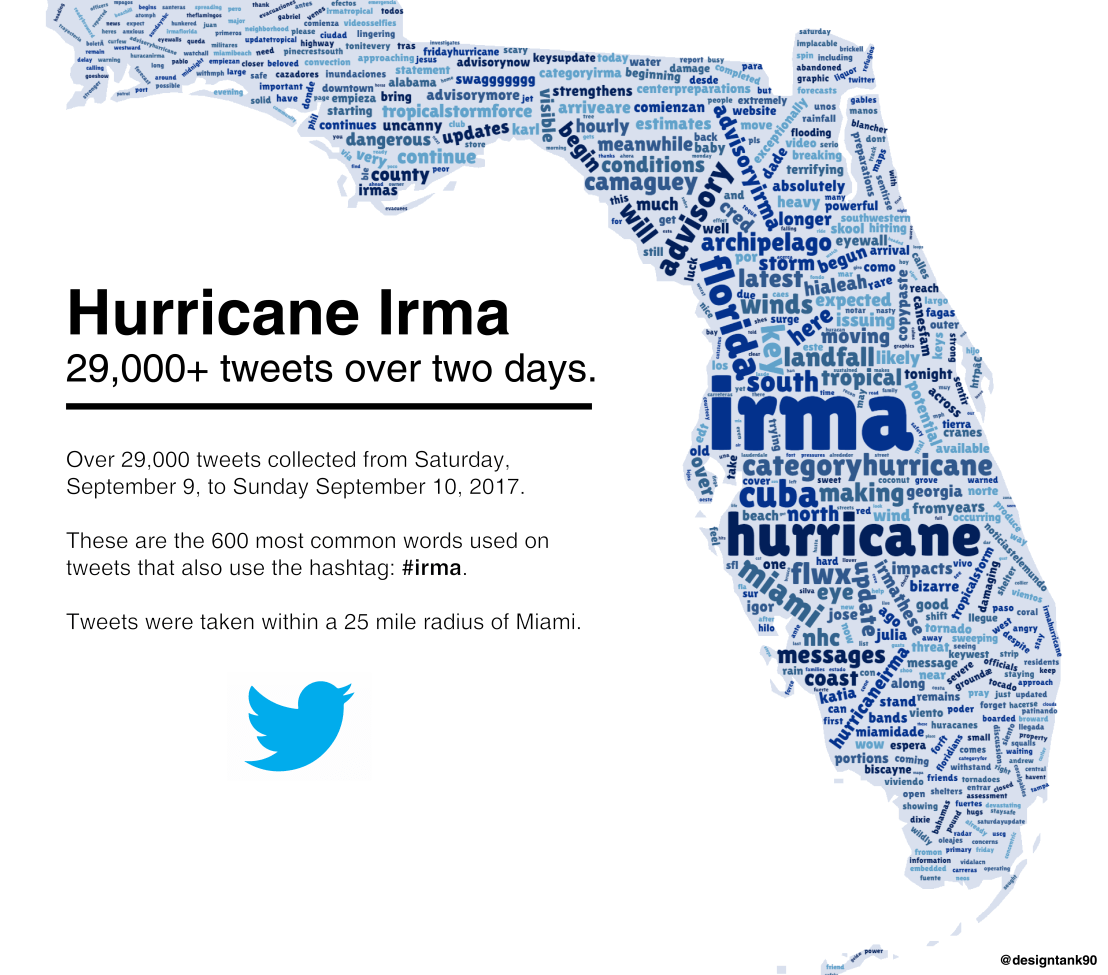
Reddit user LucasCu90 used the R package twitteR to retrieve all tweets that were sent with #Irma and a Geocode of central Miami (25 mile radius) from Saturday September 9, to Sunday September 10, 2017 (the period of Irma’s approach and initial landfall on the Florida Keys and the mainland). From the 29,000 tweets he collected, Lucas then retrieved the 600 most common words and overlaid them on a map of Florida, with their size relative to their frequency in the data. The result is quite nice!