Two Tinder Experiments: An Unequal Economy

Two Tinder Experiments: An Unequal Economy

I’ve seen a fair share of Tinder experiments come by, for instance, someone A/B-testing attractiveness with and without facial hair, but these new two posts on Medium are the best I’ve come across so far.

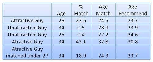
In his first experiment, this self-proclaimed worst online dater went catfishing. He made a Tinder account using stock photos of attractive and less attractive and old and young guys, looking and sampled some like ratio’s.

Basically, his conclusion was that “Tinder actually can work, but pretty much only if you are an attractive guy”

In the second experiment, the author decided to treat Tinder as an economy and study it as an (socio-)economist would:

The wealth of an economy is quantified in terms its currency. […] In Tinder the currency is “likes”. […] Wealth in Tinder is not distributed equally. Attractive guys have more wealth in the Tinder economy (get more “likes”) than unattractive guys do. […] An unequal wealth distribution is to be expected, but there is a more interesting question: What is the degree of this unequal wealth distribution and how does this inequality compare to other economies?

Original Medium Post by Worst Online Dater

The author notes some caveats of this analysis. First and foremost, the data was collected in quite an unethical way, by asking questions to 27 of the matches with the fake accounts the author set up. Moreover, self-report bias is quite likely, as it’s easy to lie on Tinder. Still, the results are quite amusing:

Basically, “the bottom 80% of men are fighting over the bottom 22% of women and the top 78% of women are fighting over the top 20% of men”

Via Medium

The Lorenz curve shows the proportion of wealth owned by the bottom x% of a population. If wealth was equally distributed the curve would be perfectly diagonal (a 45 degree slope). The steeper the slope, the less inequal an economy. The below shows the curve for a perfectly equal economy, the US economy, and the estimated Tinder economy:

Via Medium

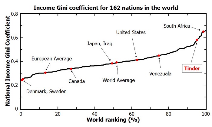
Similarly, the Gini coefficient can be used to represent the wealth equality of an economy. It ranges from 0 to 1, where 0 corresponds with perfect equality (everybody has the same wealth) and 1 corresponds with perfect inequality (one dictator with all the wealth). While most European countries, and even the US, score quite low on this Gini index, the Tinder economy is estimated to be much more towards the lower end.

Via Medium

Finally, based on the collected data, the author was able to reduce Tinder Male Attractiveness to a function of the number of likes received:

Via Medium

According to my last post, the most attractive men will be liked by only approximately 20% of all the females on Tinder. […] Unfortunately, this percentage decreases rapidly as you go down the attractiveness scale. According to this analysis a man of average attractiveness can only expect to be liked by slightly less than 1% of females (0.87%). This equates to 1 “like” for every 115 females.

The good news is that if you are only getting liked by a few girls on Tinder you shouldn’t take it personally. You aren’t necessarily unattractive. You can be of above average attractiveness and still only get liked by a few percent of women on Tinder. The bad news is that if you aren’t in the very upper echelons of Tinder wealth (i.e. attractiveness) you aren’t likely to have much success using Tinder. You would probably be better off just going to a bar or joining some coed recreational sports team.

Original Medium Post by Worst Online Dater

Python for R users

Python for R users

Wanting to broaden your scope and learn a new programming language? This great workshop was given at EARL 2018 by Mango Solutions and helps R programmers transition into Python building on their existing R knowledge. The workshop includes exercises that introduce you to the key concepts of Python and some of its most powerful packages for data science, including numpy, pandas, sklearn, and seaborn.

Have a look at the associated workshop guide that walk you through the assignments, or at the github repo with all materials in Jupyter notebooks.

E-Book: Probabilistic Programming & Bayesian Methods for Hackers

E-Book: Probabilistic Programming & Bayesian Methods for Hackers

The Bayesian method is the natural approach to inference, yet it is hidden from readers behind chapters of slow, mathematical analysis. Nevertheless, mathematical analysis is only one way to “think Bayes”. With cheap computing power, we can now afford to take an alternate route via probabilistic programming.

Cam Davidson-Pilon wrote the book Bayesian Methods for Hackers as a introduction to Bayesian inference from a computational and understanding-first, mathematics-second, point of view.

The book is available via Amazon, but you can access an online e-book for free. There’s also an associated GitHub repo.

The book explains Bayesian principles with code and visuals. For instance:

%matplotlib inline
from IPython.core.pylabtools import figsize
import numpy as np
from matplotlib import pyplot as plt
figsize(11, 9)

import scipy.stats as stats

dist = stats.beta
n_trials = [0, 1, 2, 3, 4, 5, 8, 15, 50, 500]
data = stats.bernoulli.rvs(0.5, size=n_trials[-1])
x = np.linspace(0, 1, 100)

for k, N in enumerate(n_trials):
    sx = plt.subplot(len(n_trials)/2, 2, k+1)
    plt.xlabel("$p$, probability of heads") \
        if k in [0, len(n_trials)-1] else None
    plt.setp(sx.get_yticklabels(), visible=False)
    heads = data[:N].sum()
    y = dist.pdf(x, 1 + heads, 1 + N - heads)
    plt.plot(x, y, label="observe %d tosses,\n %d heads" % (N, heads))
    plt.fill_between(x, 0, y, color="#348ABD", alpha=0.4)
    plt.vlines(0.5, 0, 4, color="k", linestyles="--", lw=1)

    leg = plt.legend()
    leg.get_frame().set_alpha(0.4)
    plt.autoscale(tight=True)


plt.suptitle("Bayesian updating of posterior probabilities",
             y=1.02,
             fontsize=14)

plt.tight_layout()

I can only recommend you start with the online version of Bayesian Methods for Hackers, but note that the print version helps sponsor the author ánd includes some additional features:

  • Additional Chapter on Bayesian A/B testing
  • Updated examples
  • Answers to the end of chapter questions
  • Additional explanation, and rewritten sections to aid the reader.

If you’re interested in learning more about Bayesian analysis, I recommend these other books:

Helpful resources for A/B testing

Helpful resources for A/B testing

Brandon Rohrer — (former) data scientist at Microsoft, iRobot, and Facebook — asked his network on Twitter and LinkedIn to share their favorite resources on A/B testing. It produced a nice list, which I summarized below.

The order is somewhat arbitrary, and somewhat based on my personal appreciation of the resources.

Cover image via Optimizely

Putting R in Production, by Heather Nolis & Mark Sellors

Putting R in Production, by Heather Nolis & Mark Sellors

It is often said that R is hard to put into production. Fortunately, there are numerous talks demonstrating the contrary.

Here’s one by Heather Nolis, who productionizes R models at T-Mobile. Her teams even shares open-source version of some of their productionized Tensorflow models on github. Read more about that model here.

There’s another great talk on the RStudio website. In this talk, Mark Sellors discusses some of the misinformation around the idea of what “putting something into production” actually means, and provides some tips on overcoming obstacles.

Cover image via Fotolia.

5 Quick Tips for Coding in the Classroom, by Kelly Bodwin

5 Quick Tips for Coding in the Classroom, by Kelly Bodwin

Kelly Bodwin is an Assistant Professor of Statistics at Cal Poly (San Luis Obispo) and teaches multiple courses in statistical programming. Based on her experiences, she compiled this great shortlist of five great tips to teach programming.

Kelly truly mentions some best practices, so have a look at the original article, which she summarized as follows:

1. Define your terms

Establish basic coding vocabulary early on.

  • What is the console, a script, the environment?
  • What is a function a variable, a dataframe?
  • What are strings, characters, and integers?

2. Be deliberate about teaching versus bypassing peripheral skills

Use tools like RStudio Cloud, R Markdown, and the usethis package to shelter students from setup.

Personally, this is what kept me from learning Python for a long time — the issues with starting up.

Kelly provides this personal checklist of peripherals skills including which ones she includes in her introductory courses:

Course TypeInstall/Update R and RStudioR Markdown fluencyPackage managementData managementFile and folder organizationGitHub
Intro Stat for Non-Majors⚠️⚠️
Intro Stat for Majors⚠️⚠️⚠️⚠️
Advanced Statistics⚠️⚠️
Intro to Statistical Computation

✅ = required course skill
⚠️ = optional, proceed with caution
❌ = avoid entirely
via https://teachdatascience.com/teaching_programming_tips/

3. Read code like English

The best way to debug is to read your process out loud as a sentence.

Basically Kelly argues that you should learn students to be able to translate their requirements into (R) code.

When you continuously read out your code as step-by-step computer instructions, students will learn to translate their own desires to computer instructions.

4. Require good coding practices from Day One

Kelly refers to this great talk by Jenny Bryan on “good” code and how to recognize it.

Kelly’s personal best practice included:

  • Clear code formatting
  • Object names follow consistent conventions
  • Lack of unnecessary code repetition
  • Reproducibility
  • Unit tests before large calculations
  • Commenting and/or documentation

For more R style guides, see my R resources overview.

5. Leave room for creativity

Open-ended questions (like “here’s a dataset, do a cool analysis“) let students explore and shine.


Large parts of the above were copied from this original article by Kelly Boldwin. I highly recommend you have a look at the original, and at the website hosting it: teachdatascience.com

Cover picture by freecodecamp.org.