Tag: API

Become a Data Science Professional

Amit Ness gathered an impressive list of learning resources for becoming a data scientist.

It’s great to see that he shares them publicly on his github so that others may follow along.

But beware, this learning guideline covers a multi-year process.

Amit’s personal motto seems to be “Becoming better at data science every day“.

Completing the hyperlinked list below will take you several hundreds days at the least!

Learning Philosophy:

Index

Caselaw Access Project: Structured data of over 6 million U.S. court decisions

Case.law seems like a very interesting data source for a machine learning or text mining project:

The Caselaw Access Project (“CAP”) expands public access to U.S. law. Our goal is to make all published U.S. court decisions freely available to the public online, in a consistent format, digitized from the collection of the Harvard Law Library.
The capstone of the Caselaw Access Project is a robust set of tools which facilitate access to the cases and their associated metadata. We currently offer five ways to access the data: API, bulk downloads, search, browse, and a historical trends viewer.
https://case.law/about/

Our open-source API is the best option for anybody interested in programmatically accessing our metadata, full-text search, or individual cases.
If you need a large collection of cases, you will probably be best served by our bulk data downloads. Bulk downloads for Illinois and Arkansas are available without a login, and unlimited bulk files are available to research scholars.
https://case.law/about/

Case metadata, such as the case name, citation, court, date, etc., is freely and openly accessible without limitation. Full case text can be freely viewed or downloaded but you must register for an account to do so, and currently you may view or download no more than 500 cases per day. In addition, research scholars can qualify for bulk data access by agreeing to certain use and redistribution restrictions. You can request a bulk access agreement by creating an account and then visiting your account page.
Access limitations on full text and bulk data are a component of Harvard’s collaboration agreement with Ravel Law, Inc. (now part of Lexis-Nexis). These limitations will end, at the latest, in March of 2024. In addition, these limitations apply only to cases from jurisdictions that continue to publish their official case law in print form. Once a jurisdiction transitions from print-first publishing to digital-first publishing, these limitations cease. Thus far, Illinois and Arkansas have made this important and positive shift and, as a result, all historical cases from these jurisdictions are freely available to the public without restriction. We hope many other jurisdictions will follow their example soon.
https://case.law/about/

A different project altogether is helping the team behind Caselaw improve its data quality:

Our data inevitably includes countless errors as part of the digitization process. The public launch of this project is only the start of discovering errors, and we hope you will help us in finding and fixing them.
Some parts of our data are higher quality than others. Case metadata, such as the party names, docket number, citation, and date, has received human review. Case text and general head matter has been generated by machine OCR and has not received human review.
You can report errors of all kinds at our Github issue tracker, where you can also see currently known issues. We particularly welcome metadata corrections, feature requests, and suggestions for large-scale algorithmic changes. We are not currently able to process individual OCR corrections, but welcome general suggestions on the OCR correction process.
https://case.law/about/

Putting R in Production, by Heather Nolis & Mark Sellors

It is often said that R is hard to put into production. Fortunately, there are numerous talks demonstrating the contrary.

Here’s one by Heather Nolis, who productionizes R models at T-Mobile. Her teams even shares open-source version of some of their productionized Tensorflow models on github. Read more about that model here.

There’s another great talk on the RStudio website. In this talk, Mark Sellors discusses some of the misinformation around the idea of what “putting something into production” actually means, and provides some tips on overcoming obstacles.

Cover image via Fotolia.

Improved Twitter Mining in R

R users have been using the twitter package by Geoff Jentry to mine tweets for several years now. However, a recent blog suggests a novel package provides a better mining tool: rtweet by Michael Kearney (GitHub).

Both packages use a similar setup and require you to do some prep-work by creating a Twitter “app” (see the package instructions). However, rtweet will save you considerable API-time and post-API munging time. This is demonstrated by the examples below, where Twitter is searched for #rstats-tagged tweets, first using twitteR, then using rtweet.

library(twitteR)

# this relies on you setting up an app in apps.twitter.com
setup_twitter_oauth(
  consumer_key = Sys.getenv("TWITTER_CONSUMER_KEY"), 
  consumer_secret = Sys.getenv("TWITTER_CONSUMER_SECRET")
)

r_folks <- searchTwitter("#rstats", n=300)

str(r_folks, 1)
## List of 300
##  $ :Reference class 'status' [package "twitteR"] with 17 fields
##   ..and 53 methods, of which 39 are  possibly relevant
##  $ :Reference class 'status' [package "twitteR"] with 17 fields
##   ..and 53 methods, of which 39 are  possibly relevant
##  $ :Reference class 'status' [package "twitteR"] with 17 fields
##   ..and 53 methods, of which 39 are  possibly relevant

str(r_folks[1])
## List of 1
##  $ :Reference class 'status' [package "twitteR"] with 17 fields
##   ..$ text         : chr "RT @historying: Wow. This is an enormously helpful tutorial by @vivalosburros for anyone interested in mapping "| __truncated__
##   ..$ favorited    : logi FALSE
##   ..$ favoriteCount: num 0
##   ..$ replyToSN    : chr(0) 
##   ..$ created      : POSIXct[1:1], format: "2017-10-22 17:18:31"
##   ..$ truncated    : logi FALSE
##   ..$ replyToSID   : chr(0) 
##   ..$ id           : chr "922150185916157952"
##   ..$ replyToUID   : chr(0) 
##   ..$ statusSource : chr "Twitter for Android"
##   ..$ screenName   : chr "jasonrhody"
##   ..$ retweetCount : num 3
##   ..$ isRetweet    : logi TRUE
##   ..$ retweeted    : logi FALSE
##   ..$ longitude    : chr(0) 
##   ..$ latitude     : chr(0) 
##   ..$ urls         :'data.frame': 0 obs. of  4 variables:
##   .. ..$ url         : chr(0) 
##   .. ..$ expanded_url: chr(0) 
##   .. ..$ dispaly_url : chr(0) 
##   .. ..$ indices     : num(0) 
##   ..and 53 methods, of which 39 are  possibly relevant:
##   ..  getCreated, getFavoriteCount, getFavorited, getId, getIsRetweet, getLatitude, getLongitude, getReplyToSID,
##   ..  getReplyToSN, getReplyToUID, getRetweetCount, getRetweeted, getRetweeters, getRetweets, getScreenName,
##   ..  getStatusSource, getText, getTruncated, getUrls, initialize, setCreated, setFavoriteCount, setFavorited, setId,
##   ..  setIsRetweet, setLatitude, setLongitude, setReplyToSID, setReplyToSN, setReplyToUID, setRetweetCount,
##   ..  setRetweeted, setScreenName, setStatusSource, setText, setTruncated, setUrls, toDataFrame, toDataFrame#twitterObj

The above operations required only several seconds to completely. The returned data is definitely usable, but not in the most handy format: the package models the Twitter API on to custom R objects. It’s elegant, but also likely overkill for most operations. Here’s the rtweet version:

library(rtweet)

# this relies on you setting up an app in apps.twitter.com
create_token(
  app = Sys.getenv("TWITTER_APP"),
  consumer_key = Sys.getenv("TWITTER_CONSUMER_KEY"), 
  consumer_secret = Sys.getenv("TWITTER_CONSUMER_SECRET")
) -> twitter_token

saveRDS(twitter_token, "~/.rtweet-oauth.rds")

# ideally put this in ~/.Renviron
Sys.setenv(TWITTER_PAT=path.expand("~/.rtweet-oauth.rds"))

rtweet_folks <- search_tweets("#rstats", n=300)

dplyr::glimpse(rtweet_folks)
## Observations: 300
## Variables: 35
## $ screen_name                     "AndySugs", "jsbreker", "__rahulgupta__", "AndySugs", "jasonrhody", "sibanjan...
## $ user_id                         "230403822", "703927710", "752359265394909184", "230403822", "14184263", "863...
## $ created_at                      2017-10-22 17:23:13, 2017-10-22 17:19:48, 2017-10-22 17:19:39, 2017-10-22 17...
## $ status_id                       "922151366767906819", "922150507745079297", "922150470382125057", "9221504090...
## $ text                            "RT:  (Rbloggers)Markets Performance after Election: Day 239  https://t.co/D1...
## $ retweet_count                   0, 0, 9, 0, 3, 1, 1, 57, 57, 103, 10, 10, 0, 0, 0, 34, 0, 0, 642, 34, 1, 1, 1...
## $ favorite_count                  0, 0, 0, 0, 0, 0, 0, 0, 0, 0, 0, 0, 0, 0, 2, 0, 0, 1, 0, 0, 0, 0, 0, 0, 0, 0,...
## $ is_quote_status                 FALSE, FALSE, FALSE, FALSE, FALSE, FALSE, FALSE, FALSE, FALSE, FALSE, FALSE, ...
## $ quote_status_id                 NA, NA, NA, NA, NA, NA, NA, NA, NA, NA, NA, NA, NA, NA, NA, NA, NA, NA, NA, N...
## $ is_retweet                      FALSE, FALSE, TRUE, FALSE, TRUE, TRUE, FALSE, TRUE, TRUE, TRUE, TRUE, TRUE, F...
## $ retweet_status_id               NA, NA, "922085241493360642", NA, "921782329936408576", "922149318550843393",...
## $ in_reply_to_status_status_id    NA, NA, NA, NA, NA, NA, NA, NA, NA, NA, NA, NA, NA, NA, NA, NA, NA, NA, NA, N...
## $ in_reply_to_status_user_id      NA, NA, NA, NA, NA, NA, NA, NA, NA, NA, NA, NA, NA, NA, NA, NA, NA, NA, NA, N...
## $ in_reply_to_status_screen_name  NA, NA, NA, NA, NA, NA, NA, NA, NA, NA, NA, NA, NA, NA, NA, NA, NA, NA, NA, N...
## $ lang                            "en", "en", "en", "en", "en", "en", "en", "en", "en", "en", "en", "en", "ro",...
## $ source                          "IFTTT", "Twitter for iPhone", "GaggleAMP", "IFTTT", "Twitter for Android", "...
## $ media_id                        NA, "922150500237062144", NA, NA, NA, NA, NA, NA, NA, NA, NA, NA, NA, NA, "92...
## $ media_url                       NA, "http://pbs.twimg.com/media/DMwi_oQUMAAdx5A.jpg", NA, NA, NA, NA, NA, NA,...
## $ media_url_expanded              NA, "https://twitter.com/jsbreker/status/922150507745079297/photo/1", NA, NA,...
## $ urls                            NA, NA, NA, NA, NA, NA, NA, NA, NA, NA, NA, NA, NA, NA, NA, NA, NA, NA, NA, N...
## $ urls_display                    "ift.tt/2xe1xrR", NA, NA, "ift.tt/2xe1xrR", NA, "bit.ly/2yAAL0M", "bit.ly/2yA...
## $ urls_expanded                   "http://ift.tt/2xe1xrR", NA, NA, "http://ift.tt/2xe1xrR", NA, "http://bit.ly/...
## $ mentions_screen_name            NA, NA, "DataRobot", NA, "historying vivalosburros", "NoorDinTech ikashnitsky...
## $ mentions_user_id                NA, NA, "622519917", NA, "18521423 304837258", "2511247075 739773414316118017...
## $ symbols                         NA, NA, NA, NA, NA, NA, NA, NA, NA, NA, NA, NA, NA, NA, NA, NA, NA, NA, NA, N...
## $ hashtags                        "rstats DataScience", "Rstats ACSmtg", "rstats", "rstats DataScience", "rstat...
## $ coordinates                     NA, NA, NA, NA, NA, NA, NA, NA, NA, NA, NA, NA, NA, NA, NA, NA, NA, NA, NA, N...
## $ place_id                        NA, NA, NA, NA, NA, NA, NA, NA, NA, NA, NA, NA, NA, NA, NA, NA, NA, NA, NA, N...
## $ place_type                      NA, NA, NA, NA, NA, NA, NA, NA, NA, NA, NA, NA, NA, NA, NA, NA, NA, NA, NA, N...
## $ place_name                      NA, NA, NA, NA, NA, NA, NA, NA, NA, NA, NA, NA, NA, NA, NA, NA, NA, NA, NA, N...
## $ place_full_name                 NA, NA, NA, NA, NA, NA, NA, NA, NA, NA, NA, NA, NA, NA, NA, NA, NA, NA, NA, N...
## $ country_code                    NA, NA, NA, NA, NA, NA, NA, NA, NA, NA, NA, NA, NA, NA, NA, NA, NA, NA, NA, N...
## $ country                         NA, NA, NA, NA, NA, NA, NA, NA, NA, NA, NA, NA, NA, NA, NA, NA, NA, NA, NA, N...
## $ bounding_box_coordinates        NA, NA, NA, NA, NA, NA, NA, NA, NA, NA, NA, NA, NA, NA, NA, NA, NA, NA, NA, N...
## $ bounding_box_type               NA, NA, NA, NA, NA, NA, NA, NA, NA, NA, NA, NA, NA, NA, NA, NA, NA, NA, NA, N...

This operation took equal to less time but provides the data in a tidy, immediately usable structure.

On the rtweet website, you can read about the additional functionalities this new package provides. For instance,ts_plot() provides a quick visual of the frequency of tweets. It’s possible to aggregate by the minute, i.e., by = "mins", or by some value of seconds, e.g.,by = "15 secs".

## Plot time series of all tweets aggregated by second
ts_plot(rt, by = "secs")

ts_filter() creates a time series-like data structure, which consists of “time” (specific interval of time determined via the by argument), “freq” (the number of observations, or tweets, that fall within the corresponding interval of time), and “filter” (a label representing the filtering rule used to subset the data). If no filter is provided, the returned data object includes a “filter” variable, but all of the entries will be blank "", indicating that no filter filter was used. Otherwise, ts_filter() uses the regular expressions supplied to the filter argument as values for the filter variable. To make the filter labels pretty, users may also provide a character vector using the key parameter.

## plot multiple time series by first filtering the data using
## regular expressions on the tweet "text" variable
rt %>%
  dplyr::group_by(screen_name) %>%
  ## The pipe operator allows you to combine this with ts_plot
  ## without things getting too messy.
  ts_plot() + 
  ggplot2::labs(
    title = "Tweets during election day for the 2016 U.S. election",
    subtitle = "Tweets collected, parsed, and plotted using `rtweet`"
  )

The developer cautions that these plots often resemble frowny faces: the first and last points appear significantly lower than the rest. This is caused by the first and last intervals of time to be artificially shrunken by connection and disconnection processes. To remedy this, users may specify trim = TRUE to drop the first and last observation for each time series.

Give rtweet a try and let me know whether you prefer it over twitter.

Geographical maps using Shazam Recognitions

Shazam is a mobile app that can be asked to identify a song by making it “listen”’ to a piece of music. Due to its immense popularity, the organization’s name quickly turned into a verb used in regular conversation (“Do you know this song? Let’s Shazam it.“). A successful identification is referred to as a Shazam recognition.

Shazam users can opt-in to anonymously share their location data with Shazam. Umar Hansa used to work for Shazam and decided to plot the geospatial data of 1 billion Shazam recognitions, during one of the company’s “hackdays“. The following wonderful city, country, and world maps are the result.

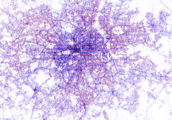
All visualisations (source) follow the same principle: Dots, representing successful Shazam recognitions, are plotted onto a blank geographical coordinate system. Can you guess the cities represented by these dots?

These first maps have an additional colour coding for operating systems. Can you guess which is which?

Blue dots represent iOS (Apple iPhones) and seem to cluster in the downtown area’s whereas red Android phones dominate the zones further from the city centres. Did you notice something else? Recall that Umar used a blank canvas, not a map from Google. Nevertheless, in all visualizations the road network is clearly visible. Umar guesses that passengers (hopefully not the drivers) often Shazam music playing in the car.

Try to guess the Canadian and American cities below and compare their layout to the two European cities that follow.

The maps were respectively of Toronto, San Fransisco, London, and Paris. It is just amazing how accurate they resemble the actual world. You have got to love the clear Atlantic borders of Europe in the world map below.

Are iPhones less common (among Shazam users) in Southern and Eastern Europe? In contrast, England and the big Japanese and Russian cities jump right out as iPhone hubs. In order to allow users to explore the data in more detail, Umar created an interactive tool comparing his maps to Google’s maps. A publicly available version you can access here (note that you can zoom in).This required quite complex code, the details of which are in his blog. For now, here is another, beautiful map of England, with (the density of) Shazam recognitions reflected by color intensity on a dark background.

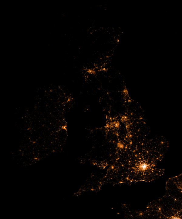
London is so crowded! New York also looks very cool. Central Park, the rivers and the bay are so clearly visible, whereas Governors Island is completely lost on this map.

If you liked this blog, please read Umar’s own blog post on this project for more background information, pieces of the JavaScript code, and the original images. If you which to follow his work, you can find him on Twitter.

EDIT — Here and here you find an alternative way of visualizing geographical maps using population data as input for line maps in the R-package ggjoy.

HD version of this world map can be found on http://spatial.ly/

Fredericton Property Values — Spot the river flowing through this city

pix2code: teaching AI to build apps

Last May, Tony Beltramelli of Ulzard Technologies presented his latest algorithm pix2code at the NIPS conference. Put simply, the algorithm looks at a picture of a graphical user interface (i.e., the layout of an app), and determines via an iterative process what the underlying code likely looks like.

Afbeeldingsresultaat voor user interface — Graphical user interface examples (Google Images)

Please watchUlzard’s pix2code demo video or the third-party summary at the bottom of this blog. My undertanding is that pix2code is based on convolutional and recurrent neural networks (long explanation video) in combination with long short-term memory (short explanation video). Based on a single input image, pix2code can generate code that is 77% accurate and it works for three of the larger platforms (i.e. iOS, Android and web-based technologies).

Obviously, this is groundbreaking technology. When further developed, pix2code not only increases the speed with which society is automated/robotized but it also further expands the automation to more complex and highly needed tasks, such as programming and web/app development.

Here you can read the full academic paper on pix2code.

Below is the official demo reviewed by another data enthusiast with commentary and some additional food for thought.