Atrebas created this extremely helpful overview page showing how to program standard data manipulation and data transformation routines in R’s famous packages dplyr and data.table.
The document has been been inspired by this stackoverflow question and by the data.table cheat sheet published by Karlijn Willems.
Resources for data.table can be found on the data.table wiki, in the data.table vignettes, and in the package documentation. Reference documents for dplyr include the dplyr cheat sheet, the dplyr vignettes, and the package documentation.
A receiver operating characteristic (ROC) curve displays how well a model can classify binary outcomes. An ROC curve is generated by plotting the false positive rate of a model against its true positive rate, for each possible cutoff value. Often, the area under the curve (AUC) is calculated and used as a metric showing how well a model can classify data points.
If you’re interest in learning more about ROC and AUC, I recommend this short Medium blog, which contains this neat graphic:
Dariya Sydykova, graduate student at the Wilke lab at the University of Texas at Austin, shared some great visual animations of how model accuracy and model cutoffs alter the ROC curve and the AUC metric. The quotes and animations are from the associated github repository.
ROC & AUC
The plot on the left shows the distributions of predictors for the two outcomes, and the plot on the right shows the ROC curve for these distributions. The vertical line that travels left-to-right is the cutoff value. The red dot that travels along the ROC curve corresponds to the false positive rate and the true positive rate for the cutoff value given in the plot on the left.
The traveling cutoff demonstrates the trade-off between trying to classify one outcome correctly and trying to classify the other outcome correcly. When we try to increase the true positive rate, we also increase the false positive rate. When we try to decrease the false positive rate, we decrease the true positive rate.
The shape of an ROC curve changes when a model changes the way it classifies the two outcomes.
The animation [below] starts with a model that cannot tell one outcome from the other, and the two distributions completely overlap (essentially a random classifier). As the two distributions separate, the ROC curve approaches the left-top corner, and the AUC value of the curve increases. When the model can perfectly separate the two outcomes, the ROC curve forms a right angle and the AUC becomes 1.
Precision-Recall
Two other metrics that are often used to quantify model performance are precision and recall.
Precision (also called positive predictive value) is defined as the number of true positives divided by the total number of positive predictions. Hence, precision quantifies what percentage of the positive predictions were correct: How correct your model’s positive predictions were.
Recall (also called sensitivity) is defined as the number of true positives divided by the total number of true postives and false negatives (i.e. all actual positives). Hence, recall quantifies what percentage of the actual positives you were able to identify: How sensitive your model was in identifying positives.
Dariya also made some visualizations of precision-recall curves:
Precision-recall curves also displays how well a model can classify binary outcomes. However, it does it differently from the way an ROC curve does. Precision-recall curve plots true positive rate (recall or sensitivity) against the positive predictive value (precision).
In the middle, here below, the ROC curve with AUC. On the right, the associated precision-recall curve.
Similarly to the ROC curve, when the two outcomes separate, precision-recall curves will approach the top-right corner. Typically, a model that produces a precision-recall curve that is closer to the top-right corner is better than a model that produces a precision-recall curve that is skewed towards the bottom of the plot.
Class imbalance
Class imbalance happens when the number of outputs in one class is different from the number of outputs in another class. For example, one of the distributions has 1000 observations and the other has 10. An ROC curve tends to be more robust to class imbalanace that a precision-recall curve.
In this animation [below], both distributions start with 1000 outcomes. The blue one is then reduced to 50. The precision-recall curve changes shape more drastically than the ROC curve, and the AUC value mostly stays the same. We also observe this behaviour when the other disribution is reduced to 50.
Here’s the same, but now with the red distribution shrinking to just 50 samples.
Dariya invites you to use these visualizations for educational purposes:
Please feel free to use the animations and scripts in this repository for teaching or learning. You can directly download the gif files for any of the animations, or you can recreate them using these scripts. Each script is named according to the animation it generates (i.e. animate_ROC.r generates ROC.gif, animate_SD.r generates SD.gif, etc.).
Want to learn more about the different evaluation metrics for machine learning? Here’s a nice how-to guide by Neptune.ai demonstrating different metrics applied in Python.
Having trouble understanding how to interpret distribution plots? Or struggling with Q-Q plots? Sven Halvorson penned down a visual tutorial explaining distributions using visualisations of their quantiles.
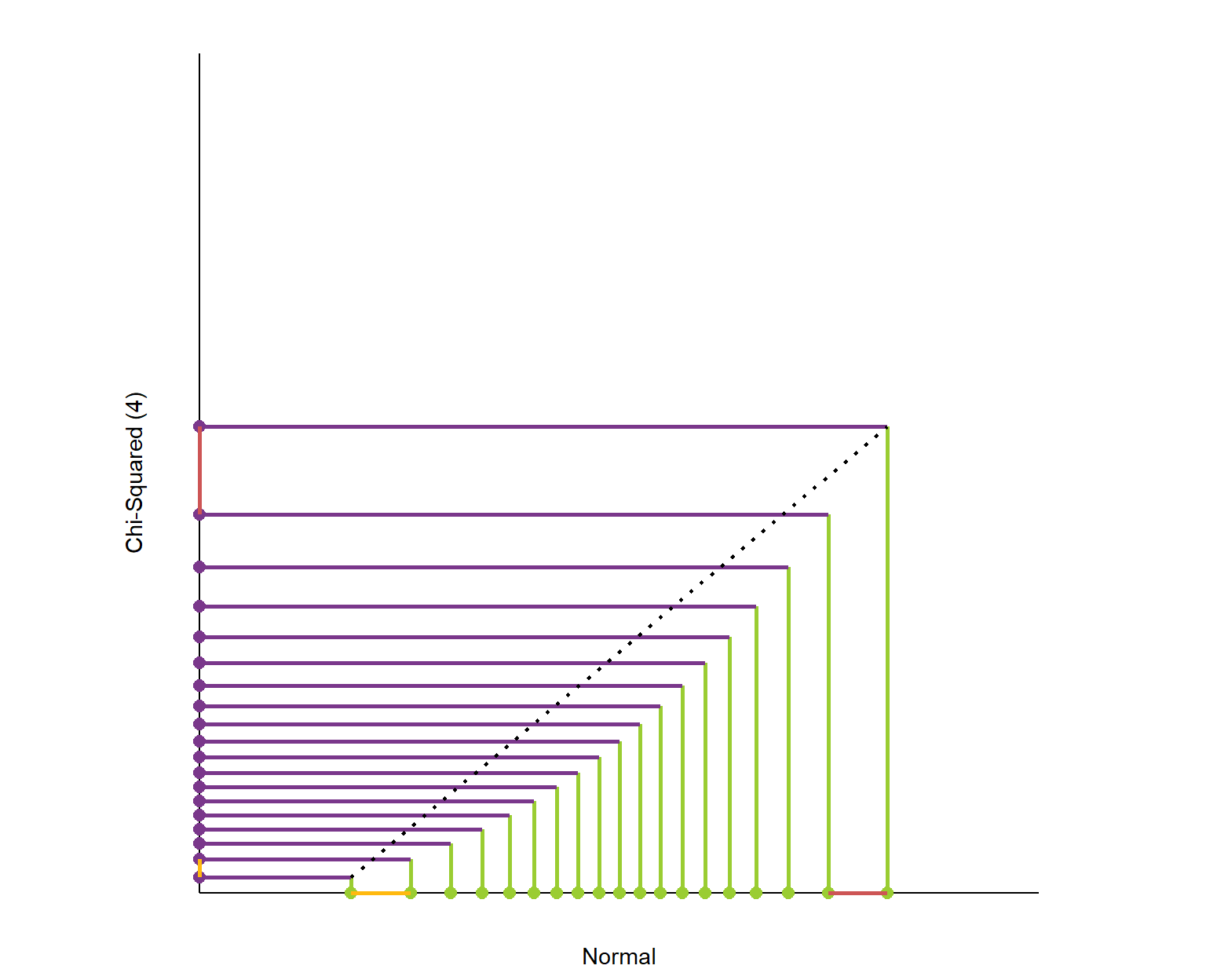
Because each slice of the distribution is 5% of the total area and the height of the graph is changing, the slices have different widths. It’s like we’re trying to cut a strange shaped cake into 20 equal pieces using parallel cuts. The slices at the center must be thinner since the distribution is denser (taller) than on the edges.
Here is the plot of matching the quantiles of the chi-squared(4) and normal distributions. I’ve again plotted these quantiles over 98% of each distribution’s range. The chi-squared distribution is skewed so its quantiles are packed into a smaller portion of its axis.
What is this graph telling us? It shows that the exchange rate between the quantiles of the two distributions is not constant.
Peter Cottle built this great interactive Git tutorial that teaches you all vital branching skills right in your browser. It’s interactive, beautiful, and very informative, introducing every concept and Git command in a step-by-step fashion.
The tutorial includes many levels that progressively teach you the Git commands you’ll need to apply version control on a daily basis:
There’s also a sandbox mode where you can interactively explore and build your own Git tree.
LearnGitBranching is a git repository visualizer, sandbox, and a series of educational tutorials and challenges. Its primary purpose is to help developers understand git through the power of visualization (something that’s absent when working on the command line). This is achieved through a game with different levels to get acquainted with the different git commands.
You can input a variety of commands into LearnGitBranching (LGB) — as commands are processed, the nearby commit tree will dynamically update to reflect the effects of each command.
Came across this awesome Youtube video that blew my mind. Definitely a handy resource if you want to explain the inner workings of neural networks. Have a look!
PyData is famous for it’s great talks on machine learning topics. This 2019 London edition, Vincent Warmerdamagain managed to give a super inspiring presentation. This year he covers what he dubs Artificial Stupidity™. You should definitely watch the talk, which includes some great visual aids, but here are my main takeaways:
Vincent speaks of Artificial Stupidity, of machine learning gone HorriblyWrong™ — an example of which below — for which Vincent elaborates on three potential fixes:
Example of a model that goes HorriblyWrong™, according to Vincent’s talk.
1. Predict Less, but Carefully
Vincent argues you shouldn’t extrapolate your predictions outside of your observed sampling space. Even better: “Not predicting given uncertainty is a great idea.” As an alternative, we could for instance design a fallback mechanism, by including an outlier detection model as the first step of your machine learning model pipeline and only predict for non-outliers.
I definately recommend you watch this specific section of Vincent’s talk because he gives some very visual and intuitive explanations of how extrapolation may go HorriblyWrong™.
Be careful! One thing we should maybe start talking about to our bosses: Algorithms merely automate, approximate, and interpolate. It’s the extrapolation that is actually kind of dangerous.
Vincent Warmerdam @ Pydata 2019 London
Basically, we can choose to not make automated decisions sometimes.
2. Constrain thy Features
What we feed to our models really matters. […] You should probably do something to the data going into your model if you want your model to have any sort of fairness garantuees.
Vincent Warmerdam @ Pydata 2019 London
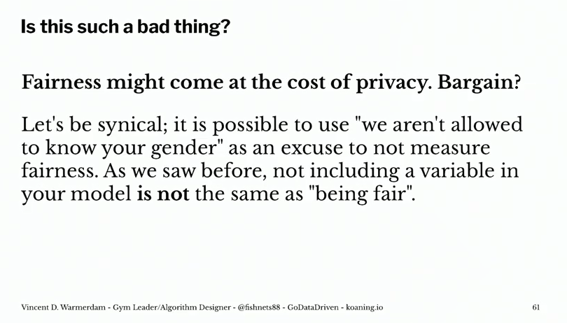
Often, simply removing biased features from your data does not reduce bias to the extent we may have hoped. Fortunately, Vincent demonstrates how to remove biased information from your variables by applying some cool math tricks.
Unfortunately, doing so will often result in a lesser predictive accuracy. Unsurprisingly though, as you are not closely fitting the biased data any more. What makes matters more problematic, Vincent rightfully mentions, is that corporate incentives often not really align here. It might feel that you need to pick: it’s either more accuracy or it’s more fairness.
However, there’s a nice solution that builds on point 1. We can now take the highly accurate model and the highly fair model, make predictions with both, and when these predictions differ, that’s a very good proxy where you potentially don’t want to make a prediction. Hence, there may be observations/samples where we are comfortable in making a fair prediction, whereas in most other situations we may say “right, this prediction seems unfair, we need a fallback mechanism, a human being should look at this and we should not automate this decision”.
Vincent does not that this is only one trick to constrain your model for fairness, and that fairness may often only be fair in the eyes of the beholder. Moreover, in order to correct for these biases and unfairness, you need to know about these unfair biases. Although outside of the scope of this specific topic, Vincent proposes this introduces new ethical issues:
Basically, we can choose to put our models on a controlled diet.
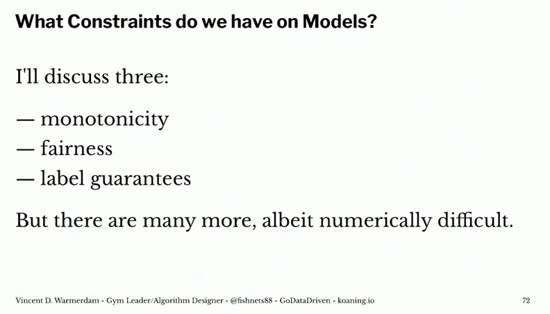
3. Constrain thy Model
Vincent argues that we should include constraints (based on domain knowledge, or common sense) into our models. In his presentation, he names a few. For instance, monotonicity, which implies that the relationship between X and Y should always be either entirely non-increasing, or entirely non-decreasing. Incorporating the previously discussed fairness principles would be a second example, and there are many more.
If we every come up with a model where more smoking leads to better health, that’s bad. I have enough domain knowledge to say that that should never happen. So maybe I should just make a system where I can say “look this one column with relationship to Y should always be strictly negative”.
Vincent Warmerdam @ Pydata 2019 London
Basically, we can integrate domain knowledge or preferences into our models.