Grant Sanderson is the owner of YouTube channel 3Blue1Brown, which aims to explain math and stats concepts in an entertaining way. Using animations, Grant grasps difficult problems and explains them in understandable language. I was already familiar with the great explanatory videos on Linear Algebra and Neural Networks, but this new video on cryptocurrencies and blockchain (below) is definitely one of the best explanations of Bitcoin I’ve seen so far:
Multilevel models (also known as hierarchical linear models, nested data models, mixed models, random coefficient, random-effects models, random parameter models, or split-plot designs) are statistical models of parameters that vary at more than one level (Wikipedia). They are very useful in Social Sciences, where we are often interested in individuals that reside in nations, organizations, teams, or other higher-level units. Next to their individuals characteristics, the characteristics of these units they belong to may also have effects. To take into account effects from variables residing at multiple levels, we can use multilevel or hierarchical models.
If you want to practice hierarchical modeling in R, I recommend the lesson by Page Paccini (first video) or the more elaborate video series by Statistics of DOOM (second):
# retrieve data filelink="https://gist.githubusercontent.com/maartenzam/787498bbc07ae06b637447dbd430ea0a/raw/9a9dafafb44d8990f85243a9c7ca349acd3a0d07/worldtilegrid.csv"geodata<-read.csv(link)%>%as.tibble()# load in geodatastr(geodata)# examine geodata
A regular expression (regex or regexp for short) is a special text string for describing a search pattern. You can think of regular expressions as wildcards on steroids. You are probably familiar with wildcard notations such as *.txt to find all text files in a file manager. The regex equivalent is .*\.txt$.
Last week I posted a first tutorial on Regular Expressions in R and I am working its sequels. You may find additional resources on Regular Expressions in the learning overviews (R, Python, Data Science).
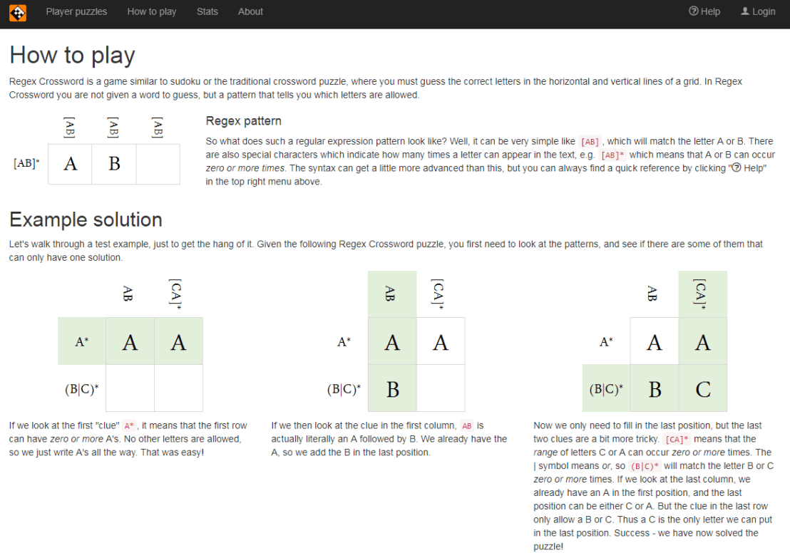
Today I came across this website of Regular Expression Crosswords, which proves a great resource to playfully master regular expression. All puzzles are validated live using the JavaScript regex engine. The figure below explains how it works
Via the links below you can jump puzzles that matches your expertise level:
For newcomers, R code can look like old Egyptian hieroglyphs with its weird operators (%in%,<-,||, or %/%). The R language has been said to have a steep learning curve and although there are many introductory courses and books (see R Resources), it’s hard to decide where to start.
Fortunately, I am here to help! The below is a six-step guide on how to learning R, using only open access (i.e., free!) materials.
Although oriented at complete newcomers, it will have you writing your own practical scripts and programs in no time: just start at #1 and work your way to coding mastery!
If you already feel comfortable with the basics of R — or don’t like basics — you can start at #5 and jump into practical learning via the tidyverse.
Good luck!!!
Step 1: An R Folder (15 min)
Create a directory for your R learning stuff somewhere on your computer. Download this (very) short introduction to R by Paul Torfs and Claudia Bauer and store it in that folder. Now read the introduction and follow the steps. It will help you install all R software on your own computer and familiarize you with the standard data types.
Now you’re ready to really start learning and we’re going to accelerate via swirl. Open up your RStudio and enter the two lines of code below in your console window.
install.packages('swirl') #download swirl package
library(swirl) #load in swirl package
swirl (webpage) will automatically start and after a couple of prompts you will be able to choose the learning course called 1: R Programming: The basics of programming in R (see below). This course consists of 15 modules via which you will master the basics of R in the environment itself. Start with module 1 and complete between one to three modules per day, so that you finish the swirl course in a week.
Starting up swirl in RStudioswirl’s R 4 learning courses and the 15 modules belonging to the basics of R programming course
Step 4: A Pirate’s Guide to R (10h)
OK, you should now be familiar with the basics of R. However, knowledge is crystallized via repetition. I therefore suggest, you walk through the book YaRrr! The Pirate’s Guide to R (Phillips, 2017) starting in chapter 3. It’s a fun book and will provide you with more knowledge on how to program custom functions, loops, and some basic statistical modelling techniques – the thing R was actually designed for.
Step 5: R for Data Science (16h)
By now, you can say you might say you are an adapt R programmer with statistical modelling experience. However, you have been working with base R functions mostly, knowledge of which is a must-have to really understand the language. In practice, R programmers rely strongly on developed packages nevertheless. A very useful group of packages is commonly referred to as the tidyverse. You will be amazed at how much this set of packages simplifies working in R. The next step therefore, is to work through the book R for Data Science (Grolemund & Wickham, 2017) (hardcopy here).
Step 6: Specialize (∞)
You are now several steps and a couple of weeks further. You possess basic knowledge of the R language, know how to write scripts in RStudio, are capable of programming in base R as well as using the advanced functionality of the tidyverse, and you have even made a start with some basic statistical modelling.
It’s time to set you loose in the wonderful world of the R community. If you had not done this earlier, you should get accounts on Stack Overflow and Cross Validated. You might also want to subscribe to the R Help Mailing List, R Bloggers, and to my website obviously.
Join 385 other subscribers
On Twitter, have a look at #rstats and, on reddit, subscribe to the rstats, rstudio, and statistics threads. At this time, I can’t but advise you to return to the R Resources Overview and to continue broadening your R programming skills. Pick materials in the area that interests you:
Last month, a video by 3Blue1Brown has been trending on YouTube, accumulating already over a quarter of a million views. It only lasts 10 minutes but provides a very good and intuitive explanation of the inner workings of Neural Networks (NN):
If you still haven’t had enough, Daniel Shiffman demonstrates how to code Neural Networks in Processing (Java), and the video displays precisely what happens behind the scenes. Finally, MIT has made their AI course material open-source, and it includes two 45 minute lectures on NNs. The lecturing professor – Patrick Winston – isn’t much of a fan of these “bulldozer” algorithms. He has a stronger preference for “more sophisticated” mathematical learning through, for instance, Support Vector Machines.