Tag: lightgbm

Calibrating algorithmic predictions with logistic regression

I found this interesting blog by Guilherme Duarte Marmerola where he shows how the predictions of algorithmic models (such as gradient boosted machines, or random forests) can be calibrated by stacking a logistic regression model on top of it: by using the predicted leaves of the algorithmic model as features / inputs in a subsequent logistic model.

When working with ML models such as GBMs, RFs, SVMs or kNNs (any one that is not a logistic regression) we can observe a pattern that is intriguing: the probabilities that the model outputs do not correspond to the real fraction of positives we see in real life.
Guilherme’s in his blog post

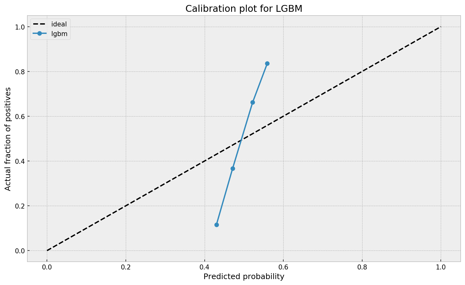
This is visible in the predictions of the light gradient boosted machine (LGBM) Guilherme trained: its predictions range only between ~ 0.45 and ~ 0.55. In contrast, the actual fraction of positive observations in those groups is much lower or higher (ranging from ~ 0.10 to ~0.85).

Motivated by sklearn’s topic Probability Calibration and the paper Practical Lessons from Predicting Clicks on Ads at Facebook, Guilherme continues to show how the output probabilities of a tree-based model can be calibrated, while simultenously improving its accuracy.

I highly recommend you look at Guilherme’s code to see for yourself what’s happening behind the scenes, but basically it’s this:

Train an algorithmic model (e.g., GBM) using your regular features (data)
Retrieve the probabilities GBM predicts
Retrieve the leaves (end-nodes) in which the GBM sorts the observations
Turn the array of leaves into a matrix of (one-hot-encoded) features, showing for each observation which leave it ended up in (1) and which not (many 0’s)
Basically, until now, you have used the GBM to reduce the original features to a new, one-hot-encoded matrix of binary features
Now you can use that matrix of new features as input for a logistic regression model predicting your target (Y) variable
Apparently, those logistic regression predictions will show a greater spread of probabilities with the same or better accuracy

Here’s a visual depiction from Guilherme’s blog, with the original GBM predictions on the X-axis, and the new logistic predictions on the Y-axis.

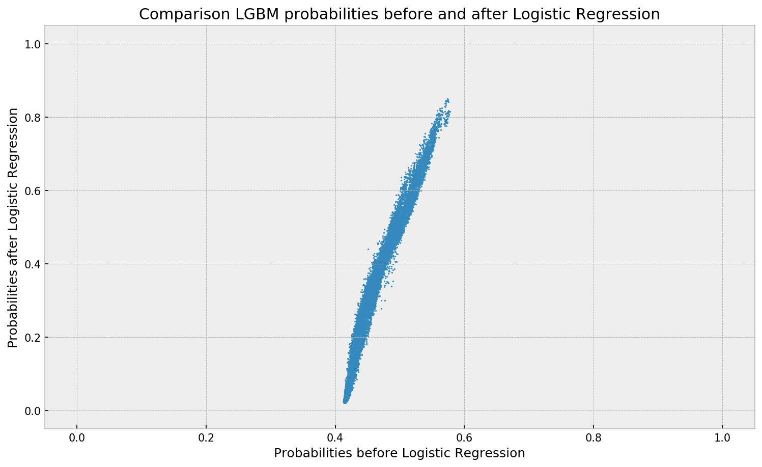
As you can see, you retain roughly the same ordering, but the logistic regression probabilities spread is much larger.

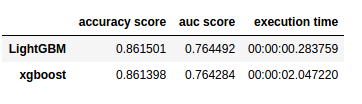
Now according to Guilherme and the Facebook paper he refers to, the accuracy of the logistic predictions should not be less than those of the original algorithmic method.

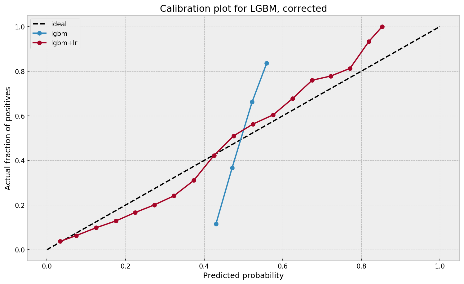
Much better. The calibration plot of lgbm+lr is much closer to the ideal. Now, when the model tells us that the probability of success is 60%, we can actually be much more confident that this is the true fraction of success! Let us now try this with the ET model.
Guilherme in https://gdmarmerola.github.io/probability-calibration/

In his blog, Guilherme shows the same process visually for an Extremely Randomized Trees model, so I highly recommend you read the original article. Also, you can find the complete code on his GitHub.

Predicting Employee Turnover at SIOP 2018

The 2018 annual Society for Industrial and Organizational Psychology (SIOP) conference featured its first-ever machine learning competition. Teams competed for several months in predicting the enployee turnover (or churn) in a large US company. A more complete introduction as presented at the conference can be found here. All submissions had to be open source and the winning submissions have been posted in this GitHub repository. The winning teams consist of analysts working at WalMart, DDI, and HumRRO. They mostly built ensemble models, in Python and/or R, combining algorithms such as (light) gradient boosted trees, neural networks, and random forest analysis.

Light GBM vs. XGBOOST in Python & R

XGBOOST stands for eXtreme Gradient Boosting. A big brother of the earlier AdaBoost, XGB is a supervised learning algorithm that uses an ensemble of adaptively boosted decision trees. For those unfamiliar with adaptive boosting algorithms, here’s a 2-minute explanation video and a written tutorial. Although XGBOOST often performs well in predictive tasks, the training process can be quite time-consuming (similar to other bagging/boosting algorithms (e.g., random forest)).

In a recent blog, Analytics Vidhya compares the inner workings as well as the predictive accuracy of the XGBOOST algorithm to an upcoming boosting algorithm: Light GBM. The blog demonstrates a stepwise implementation of both algorithms in Python. The table below reflects the main conclusion of the comparison: Although the algorithms are comparable in terms of their predictive performance, light GBM is much faster to train. With continuously increasing data volumes, light GBM, therefore, seems the way forward.

Laurae also benchmarked lightGBM against xgboost on a Bosch dataset and her results show that, on average, LightGBM (binning) is between 11x to 15x faster than xgboost (without binning):

View interactively online: https://plot.ly/~Laurae/9/

However, the differences get smaller as more threads are used due to thread inefficiencies (idle-time increases because threads are not scheduled a next task fast enough).

Light GBM is also available in R:

devtools::install_github("Microsoft/LightGBM", subdir = "R-package")

Neil Schneider tested the three algorithms for gradient boosting in R (GBM, xgboost, and lightGBM) and sums up their (dis)advantages:

GBM has no specific advantages but its disadvantages include no early stopping, slower training and decreased accuracy,
xgboost has demonstrated successful on kaggle and though traditionally slower than lightGBM, tree_method = 'hist' (histogram binning) provides a significant improvement.
lightGBM has the advantages of training efficiency, low memory usage, high accuracy, parallel learning, corporate support, and scale-ability. However, its’ newness is its main disadvantage because there is little community support.