Tag: models

Is R-squared Useless?

Coming from a social sciences background, I learned to use R-squared as a way to assess model performance and goodness of fit for regression models.

Yet, in my current day job, I nearly never use the metric any more. I tend to focus on predictive power, with metrics such as MAE, MSE, or RMSE. These make much more sense to me when comparing models and their business value, and are easier to explain to stakeholders as an added bonus.

I recently wrote about the predictive power score as an alternative to correlation analysis.

Are there similar alternatives that render R-squared useless? And why?

Here’s an interesting blog explaining the standpoints of Cosma Shalizi of Carnegie Mellon University:

R-squared does not measure goodness of fit.
R-squared does not measure predictive error.
R-squared does not allow you to compare models using transformed responses.
R-squared does not measure how one variable explains another.

I have never found a situation where R-squared helped at all.
Professor Cosma Shalizi (according to Clay Ford)

How most statistical tests are linear models

Jonas Kristoffer Lindeløv wrote a great visual explanation of how the most common statistical tests (t-test, ANOVA, ANCOVA, etc) are all linear models in the back-end.

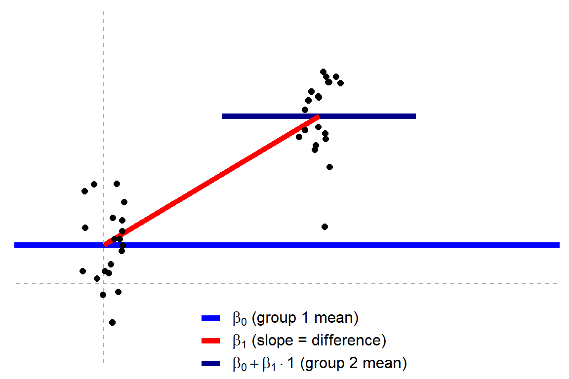
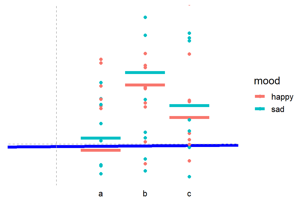
Jonas’ original blog uses R programming to visually show how the tests work, what the linear models look like, and how different approaches result in the same statistics.

George Ho later remade a Python programming version of the same visual explanation.

If I was thought statistics and methodology this way, I sure would have struggled less! Have a look yourself: https://lindeloev.github.io/tests-as-linear/

Need to save R’s lm() or glm() models? Trim the fat!

I was training a predictive model for work for use in a Shiny App. However, as the training set was quite large (700k+ obs.), the model object to save was also quite large in size (500mb). This slows down your operation significantly!

Basically, all you really need are the coefficients (and a link function, in case of glm()). However, I can imagine that you are not eager to write new custom predictions functions, but that you would rather want to rely on R’s predict.lm and predict.glm. Hence, you’ll need to save some more object information.

Via Google I came to this blog, which provides this great custom R function (below) to decrease the object size of trained generalized linear models considerably! It retains only those object data that are necessary to make R’s predict functions work.

My saved linear model went from taking up half a GB to only 27kb! That’s a 99.995% reduction!

strip_glm = function(cm) {
  cm$y = c()
  cm$model = c()
  
  cm$residuals = c()
  cm$fitted.values = c()
  cm$effects = c()
  cm$qr$qr = c()  
  cm$linear.predictors = c()
  cm$weights = c()
  cm$prior.weights = c()
  cm$data = c()
  
  
  cm$family$variance = c()
  cm$family$dev.resids = c()
  cm$family$aic = c()
  cm$family$validmu = c()
  cm$family$simulate = c()
  attr(cm$terms,".Environment") = c()
  attr(cm$formula,".Environment") = c()
  
  cm
}

Calibrating algorithmic predictions with logistic regression

I found this interesting blog by Guilherme Duarte Marmerola where he shows how the predictions of algorithmic models (such as gradient boosted machines, or random forests) can be calibrated by stacking a logistic regression model on top of it: by using the predicted leaves of the algorithmic model as features / inputs in a subsequent logistic model.

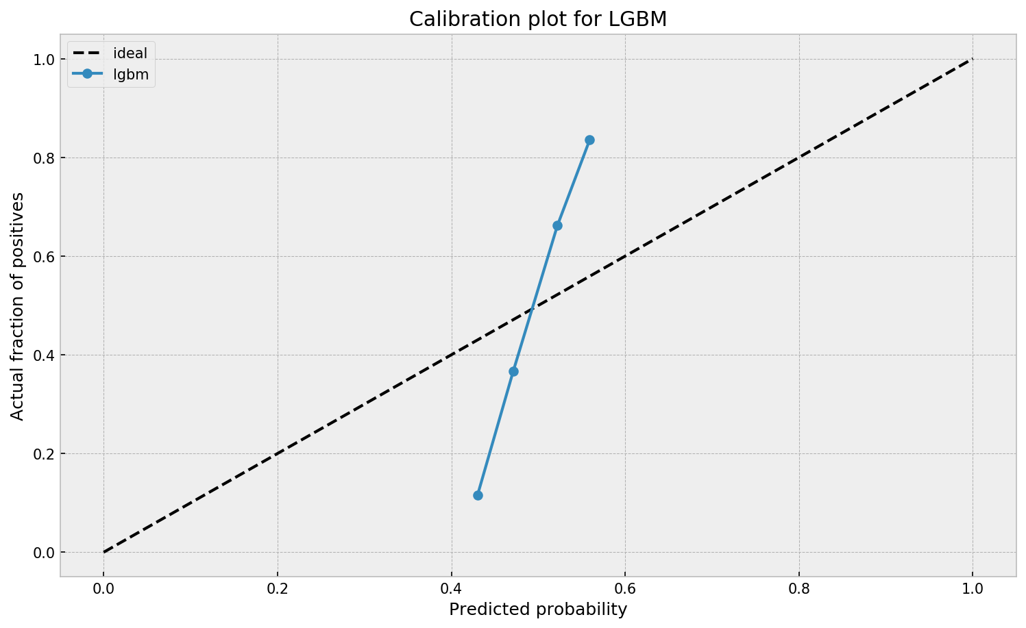
When working with ML models such as GBMs, RFs, SVMs or kNNs (any one that is not a logistic regression) we can observe a pattern that is intriguing: the probabilities that the model outputs do not correspond to the real fraction of positives we see in real life.
Guilherme’s in his blog post

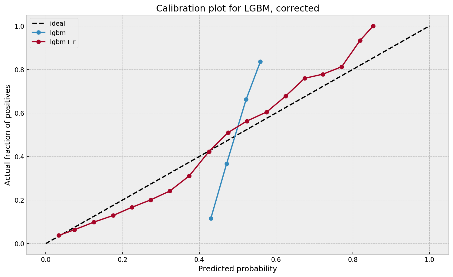
This is visible in the predictions of the light gradient boosted machine (LGBM) Guilherme trained: its predictions range only between ~ 0.45 and ~ 0.55. In contrast, the actual fraction of positive observations in those groups is much lower or higher (ranging from ~ 0.10 to ~0.85).

Motivated by sklearn’s topic Probability Calibration and the paper Practical Lessons from Predicting Clicks on Ads at Facebook, Guilherme continues to show how the output probabilities of a tree-based model can be calibrated, while simultenously improving its accuracy.

I highly recommend you look at Guilherme’s code to see for yourself what’s happening behind the scenes, but basically it’s this:

Train an algorithmic model (e.g., GBM) using your regular features (data)
Retrieve the probabilities GBM predicts
Retrieve the leaves (end-nodes) in which the GBM sorts the observations
Turn the array of leaves into a matrix of (one-hot-encoded) features, showing for each observation which leave it ended up in (1) and which not (many 0’s)
Basically, until now, you have used the GBM to reduce the original features to a new, one-hot-encoded matrix of binary features
Now you can use that matrix of new features as input for a logistic regression model predicting your target (Y) variable
Apparently, those logistic regression predictions will show a greater spread of probabilities with the same or better accuracy

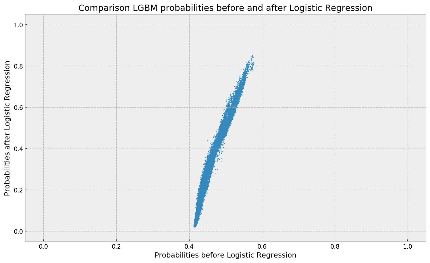
Here’s a visual depiction from Guilherme’s blog, with the original GBM predictions on the X-axis, and the new logistic predictions on the Y-axis.

As you can see, you retain roughly the same ordering, but the logistic regression probabilities spread is much larger.

Now according to Guilherme and the Facebook paper he refers to, the accuracy of the logistic predictions should not be less than those of the original algorithmic method.

Much better. The calibration plot of lgbm+lr is much closer to the ideal. Now, when the model tells us that the probability of success is 60%, we can actually be much more confident that this is the true fraction of success! Let us now try this with the ET model.
Guilherme in https://gdmarmerola.github.io/probability-calibration/

In his blog, Guilherme shows the same process visually for an Extremely Randomized Trees model, so I highly recommend you read the original article. Also, you can find the complete code on his GitHub.

Generalized Additive Models Tutorial in R, by Noam Ross

Generalized Additive Models — or GAMs in short — have been somewhat of a mystery to me. I’ve known about them, but didn’t know exactly what they did, or when they’re useful. That came to an end when I found out about this tutorial by Noam Ross.

In this beautiful, online, interactive course, Noam allows you to program several GAMs yourself (in R) and to progressively learn about the different functions and features. I am currently halfway through, but already very much enjoy it.

If you’re already familiar with linear models and want to learn something new, I strongly recommend this course!