I found this interesting blog by Guilherme Duarte Marmerola where he shows how the predictions of algorithmic models (such as gradient boosted machines, or random forests) can be calibrated by stacking a logistic regression model on top of it: by using the predicted leaves of the algorithmic model as features / inputs in a subsequent logistic model.
When working with ML models such as GBMs, RFs, SVMs or kNNs (any one that is not a logistic regression) we can observe a pattern that is intriguing: the probabilities that the model outputs do not correspond to the real fraction of positives we see in real life.
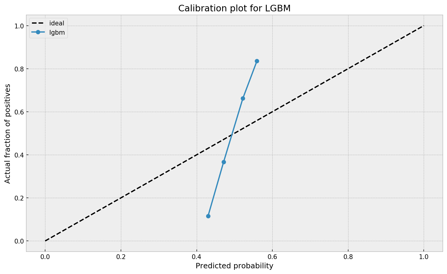
This is visible in the predictions of the light gradient boosted machine (LGBM) Guilherme trained: its predictions range only between ~ 0.45 and ~ 0.55. In contrast, the actual fraction of positive observations in those groups is much lower or higher (ranging from ~ 0.10 to ~0.85).
I highly recommend you look at Guilherme’s code to see for yourself what’s happening behind the scenes, but basically it’s this:
Train an algorithmic model (e.g., GBM) using your regular features (data)
Retrieve the probabilities GBM predicts
Retrieve the leaves (end-nodes) in which the GBM sorts the observations
Turn the array of leaves into a matrix of (one-hot-encoded) features, showing for each observation which leave it ended up in (1) and which not (many 0’s)
Basically, until now, you have used the GBM to reduce the original features to a new, one-hot-encoded matrix of binary features
Now you can use that matrix of new features as input for a logistic regression model predicting your target (Y) variable
Apparently, those logistic regression predictions will show a greater spread of probabilities with the same or better accuracy
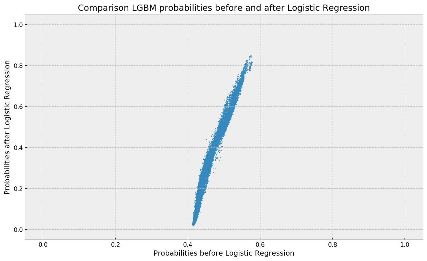
Here’s a visual depiction from Guilherme’s blog, with the original GBM predictions on the X-axis, and the new logistic predictions on the Y-axis.
As you can see, you retain roughly the same ordering, but the logistic regression probabilities spread is much larger.
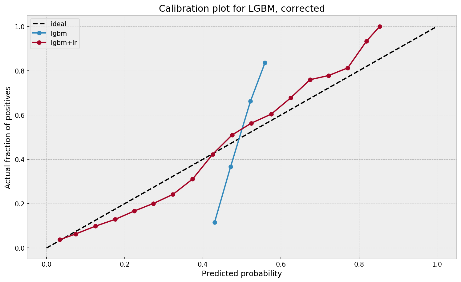
Now according to Guilherme and the Facebook paper he refers to, the accuracy of the logistic predictions should not be less than those of the original algorithmic method.
Much better. The calibration plot of lgbm+lr is much closer to the ideal. Now, when the model tells us that the probability of success is 60%, we can actually be much more confident that this is the true fraction of success! Let us now try this with the ET model.
In his blog, Guilherme shows the same process visually for an Extremely Randomized Trees model, so I highly recommend you read the original article. Also, you can find the complete code on his GitHub.
Lisa Charlotte Rost of DataWrapper often writes about data visualization and lately she has focused on the (im)proper use of color in visualization. In this recent blog, she gives a bunch of great tips and best practices, some of which I copied below:
Adam Geitgey likes to write about computers and machine learning. He explains machine learning as “generic algorithms that can tell you something interesting about a set of data without you having to write any custom code specific to the problem. Instead of writing code, you feed data to the generic algorithm and it builds its own logic based on the data.” (Part 1)
Adam’s visual explanation of two machine learning applications (original from Part 1)
In the fourth part of his series on machine learning Adam touches on Facial Recognition. Facebook is one of the companies using such algorithms in real-time, allowing them to recognize your friends’ faces after you’ve tagged them only a few times. Facebook reports they recognize faces with 97% accuracy, which is comparable to our own, human facial recognition abilities!
Facebook’s algorithms recognizing and automatically tagging Adam’s family. Helpful or creepy? (original from Part 4)
Adam decided to put up a challenge: would a facial recognition algorithm be able to distinguish Will Ferrell (famous actor) from Chad Smith (famous rock musician)? Indeed, these two celebrities look very much alike:
If you want to train such an algorithm, Adam explain, you need to overcome a series of related problems:
First, look at a picture and find all the faces in it
Second, focus on each face and be able to understand that even if a face is turned in a weird direction or in bad lighting, it is still the same person.
Third, be able to pick out unique features of the face that you can use to tell it apart from other people— like how big the eyes are, how long the face is, etc.
Finally, compare the unique features of that face to all the people you already know to determine the person’s name.
How the facial recognition algorithm steps might work (original from Part 4)
To detect the faces, Adam used Histograms of Oriented Gradients (HOG). All input pictures were converted to black and white (because color is not needed) and then every single pixel in our image is examined, one at a time. Moreover, for every pixel, the algorithm examined the pixels directly surrounding it:
Illustration of the algorithm as it would take in a black and white photo of Will Ferrel (original from Part 4)
The algorithm then checks, for every pixel, in which direction the picture is getting darker and draws an arrow (a gradient) in that direction.
Illustration of how algorithm would reduce a black and white photo of Will Ferrel to gradients (original from Part 4)
However, to do this for every single pixel would require too much processing power, so Adam broke up pictures in 16 by 16 pixel squares. The result is a very simple representation that does capture the basic structure of the original face, based on which we can now spot faces in pictures. Moreover, because we used gradients, the result will be similar regardless of the lighting of the picture.
The original image turned into a HOG representation (original from Part 4)
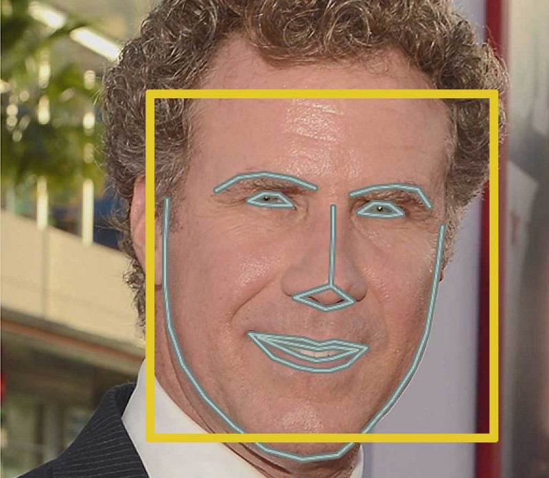
Now that the computer can spot faces, we need to make sure that it knows that two perspectives of the same face represent the same person. Adam uses landmarks for this: 68 specific points that exist on every face. An algorithm can then be trained to find these points on any face:
The 68 points on the image of Will Ferrell (original from Part 4)
Now the computer knows where the chin, the mouth and the eyes are, the image can be scaled and rotated to center it as best as possible:
The image of Will Ferrell transformed (original from Part 4)
Adam trained a Deep Convolutional Neural Network to generate 128 measurements for each face that best distinguish it from faces of other people. This network needs to train for several hours, going through thousands and thousands of face pictures. If you want to try this step yourself, Adam explains how to run OpenFace’s lua script. This study at Google provides more details, but it basically looks like this:
The training process visualized (original from Part 4)
After hours of training, the neural net will output 128 numbers accurately representing the specific face put in. Now, all you need to do is check which face in your database is most closely resembled by those 128 numbers, and you have your match! Many algorithms can do this final check, and Adam trained a simple linear SVM classifier on twenty pictures of Chad Smith, Will Ferrel, and Jimmy Falon (the host of a talkshow they both visited).
In the end, Adam’s machine had learned to distinguish these three people – two of whom are nearly indistinguishable with the human eye – in real-time:
Adam Geitgey’s facial recognition algorithm in action: providing real time classifications of the faces of lookalikes Chad Smith and Will Ferrel at Jimmy Falon’s talk show (original from Part 4)