Thanks to Sebastian Raschka I am able to share this great GitHub overview page of relevant graph classification techniques, and the scientific papers behind them. The overview divides the algorithms into four groups:
As well as a link to relevant graph classification benchmark datasets.
"Awesome Graph Classification" — A collection of graph classification methods, covering embedding, deep learning, graph kernel, and factorization papers with reference implementations https://t.co/ugpL3xSvf1
I’ve seen some uses of reinforcement learning and generative algorithms for architectural purposes already, like these evolving blueprints for school floorplans. However, this new application called ArchiGAN blew me away!
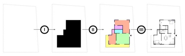
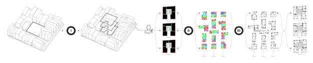
ArchiGAN (try here) was made by Stanislas Chaillou as a Harvard master’s thesis project. The program functions in three steps:
building footprint massing
program repartition
furniture layout
Stanislas’ three generation steps
Each of these three steps uses a TensorFlow Pix2Pix GAN-model (Christopher Hesse’s implementation) in the back-end, and their combination makes for a entire apartment building “generation stack” — according to Stanislas — which also allows for user input at each step.
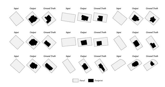
The design of a building can be inferred from the piece of land it stands on. Hence, Stanislas fed his first model using GIS-data (Geographic Information System) from the city of Boston in order to generate typical footprints based on parcel shapes.
The inputs and outputs of model I
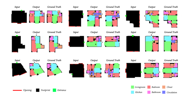
Stanislas’ second model was responsible for repartition and fenestration (the placement of windows and doors). This GAN took the footprint of the building (the output of model I) as input, along with the position of the entrance door (green square), and the positions of the user-specified windows.
Stanislas used a database of 800+ plans of apartments for training. To visualize the output, rooms are color-coded and walls and fenestration are blackened.
The inputs and outputs of model II
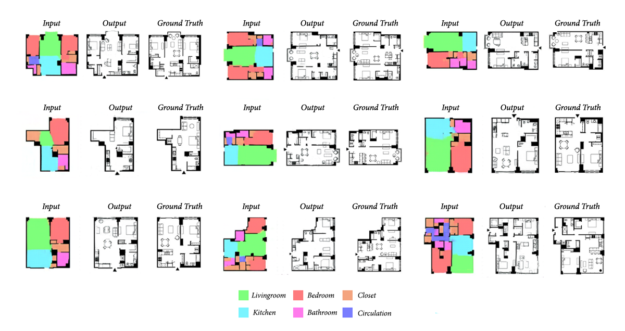
Finally, in the third model, the rooms are filled with appropriate furniture. What training data Stanislas has used here, he did not specify in the original blog.
The inputs and outputs of model III
Now, to put all things together, Stanislas created a great interactive tool you can play with yourself. The original NVIDEA blog contains some great GIFs of the tool being used:
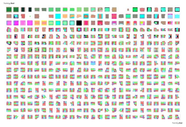
Stanislas’ GAN-models progressively learned to design rooms and realistically position doors and windows. It took about 250 iterations to get some realistic floorplans out of the algorithm. Here’s how an example learning sequence looked like:
Visualization of the training process
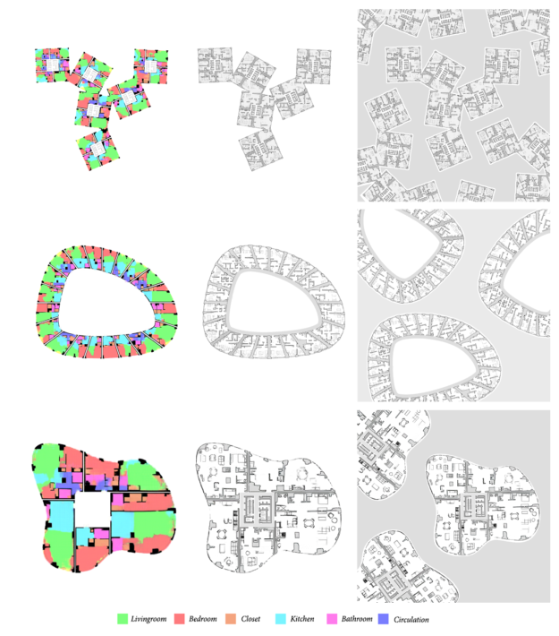
Now, Stanislas was not done yet. He also scaled the utilization of GANs to design whole apartment buildings. Here, he chains the models and processes multiple units as single images at each step.
Generating whole appartment blocks using ArchiGAN
Stanislas did other cool things to improve the flexibility of his ArchiGAN models, about which you can read more in the original blog. Let these visuals entice you to read more:
ArchiGAN scaled to handle whole appartment blocks and neighborhoods.
I believe a statistical approach to design conception will shape AI’s potential for Architecture. This approach is less deterministic and more holistic in character. Rather than using machines to optimize a set of variables, relying on them to extract significant qualities and mimicking them all along the design process represents a paradigm shift.
I am so psyched about these innovative applications of machine learning, so please help me give Stanislas the attention and credit he deserved.
Currently, Stanislas is Data Scientist & Architect at Spacemaker.ai. Read more about him in his NVIDEA developer bio here. He recently published a sequence of articles, laying down the premise of AI’s intersection with Architecture. Read here about the historical background behind this significant evolution, to be followed by AI’s potential for floor plan design, and for architectural style analysis & generation.
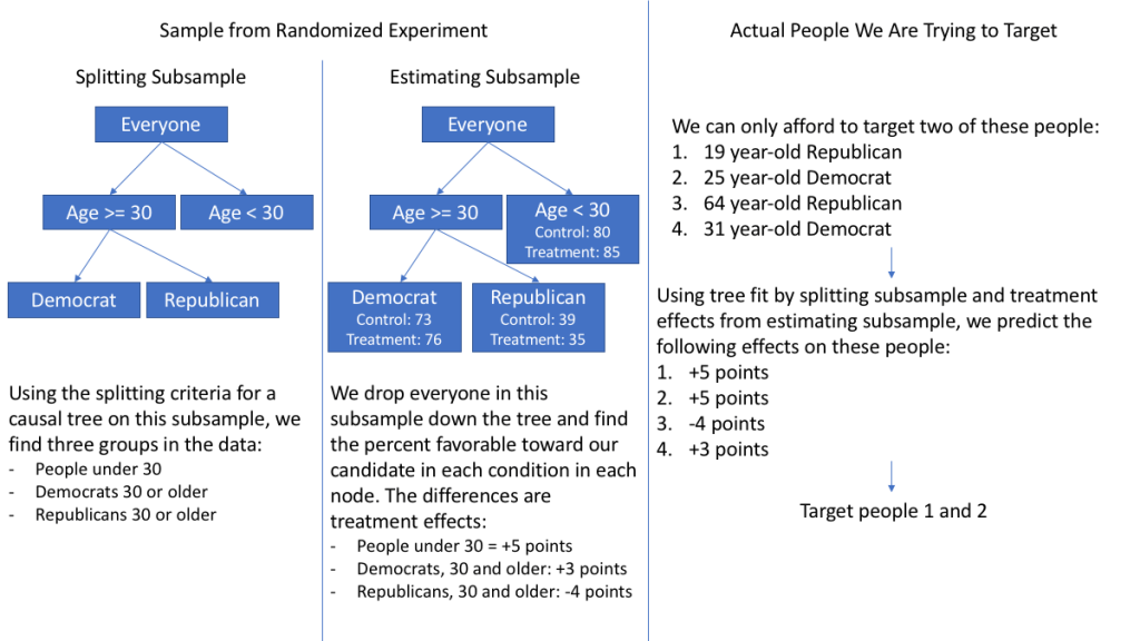
I stumbled accros this incredibly interesting read by Mark White, who discusses the (academic) theory behind, inner workings, and example (R) applications of causal random forests:
These so-called “honest” forests seem a great technique to identify opportunities for personalized actions: think of marketing, HR, medicine, healthcare, and other personalized recommendations. Note that an experimental setup for data collection is still necessary to gather the right data for these techniques.
Jared Wilber posted this great walkthrough where he codes a simple R data pipeline using purrr and tidyr to train a large variety of models and methods on the same base data, all in a non-repetitive, reproducible, clean, and thus tidy fashion. Really impressive workflow!
A receiver operating characteristic (ROC) curve displays how well a model can classify binary outcomes. An ROC curve is generated by plotting the false positive rate of a model against its true positive rate, for each possible cutoff value. Often, the area under the curve (AUC) is calculated and used as a metric showing how well a model can classify data points.
If you’re interest in learning more about ROC and AUC, I recommend this short Medium blog, which contains this neat graphic:
Dariya Sydykova, graduate student at the Wilke lab at the University of Texas at Austin, shared some great visual animations of how model accuracy and model cutoffs alter the ROC curve and the AUC metric. The quotes and animations are from the associated github repository.
ROC & AUC
The plot on the left shows the distributions of predictors for the two outcomes, and the plot on the right shows the ROC curve for these distributions. The vertical line that travels left-to-right is the cutoff value. The red dot that travels along the ROC curve corresponds to the false positive rate and the true positive rate for the cutoff value given in the plot on the left.
The traveling cutoff demonstrates the trade-off between trying to classify one outcome correctly and trying to classify the other outcome correcly. When we try to increase the true positive rate, we also increase the false positive rate. When we try to decrease the false positive rate, we decrease the true positive rate.
The shape of an ROC curve changes when a model changes the way it classifies the two outcomes.
The animation [below] starts with a model that cannot tell one outcome from the other, and the two distributions completely overlap (essentially a random classifier). As the two distributions separate, the ROC curve approaches the left-top corner, and the AUC value of the curve increases. When the model can perfectly separate the two outcomes, the ROC curve forms a right angle and the AUC becomes 1.
Precision-Recall
Two other metrics that are often used to quantify model performance are precision and recall.
Precision (also called positive predictive value) is defined as the number of true positives divided by the total number of positive predictions. Hence, precision quantifies what percentage of the positive predictions were correct: How correct your model’s positive predictions were.
Recall (also called sensitivity) is defined as the number of true positives divided by the total number of true postives and false negatives (i.e. all actual positives). Hence, recall quantifies what percentage of the actual positives you were able to identify: How sensitive your model was in identifying positives.
Dariya also made some visualizations of precision-recall curves:
Precision-recall curves also displays how well a model can classify binary outcomes. However, it does it differently from the way an ROC curve does. Precision-recall curve plots true positive rate (recall or sensitivity) against the positive predictive value (precision).
In the middle, here below, the ROC curve with AUC. On the right, the associated precision-recall curve.
Similarly to the ROC curve, when the two outcomes separate, precision-recall curves will approach the top-right corner. Typically, a model that produces a precision-recall curve that is closer to the top-right corner is better than a model that produces a precision-recall curve that is skewed towards the bottom of the plot.
Class imbalance
Class imbalance happens when the number of outputs in one class is different from the number of outputs in another class. For example, one of the distributions has 1000 observations and the other has 10. An ROC curve tends to be more robust to class imbalanace that a precision-recall curve.
In this animation [below], both distributions start with 1000 outcomes. The blue one is then reduced to 50. The precision-recall curve changes shape more drastically than the ROC curve, and the AUC value mostly stays the same. We also observe this behaviour when the other disribution is reduced to 50.
Here’s the same, but now with the red distribution shrinking to just 50 samples.
Dariya invites you to use these visualizations for educational purposes:
Please feel free to use the animations and scripts in this repository for teaching or learning. You can directly download the gif files for any of the animations, or you can recreate them using these scripts. Each script is named according to the animation it generates (i.e. animate_ROC.r generates ROC.gif, animate_SD.r generates SD.gif, etc.).
Want to learn more about the different evaluation metrics for machine learning? Here’s a nice how-to guide by Neptune.ai demonstrating different metrics applied in Python.
Came across this awesome Youtube video that blew my mind. Definitely a handy resource if you want to explain the inner workings of neural networks. Have a look!