Category: statistics

ROC, AUC, precision, and recall visually explained

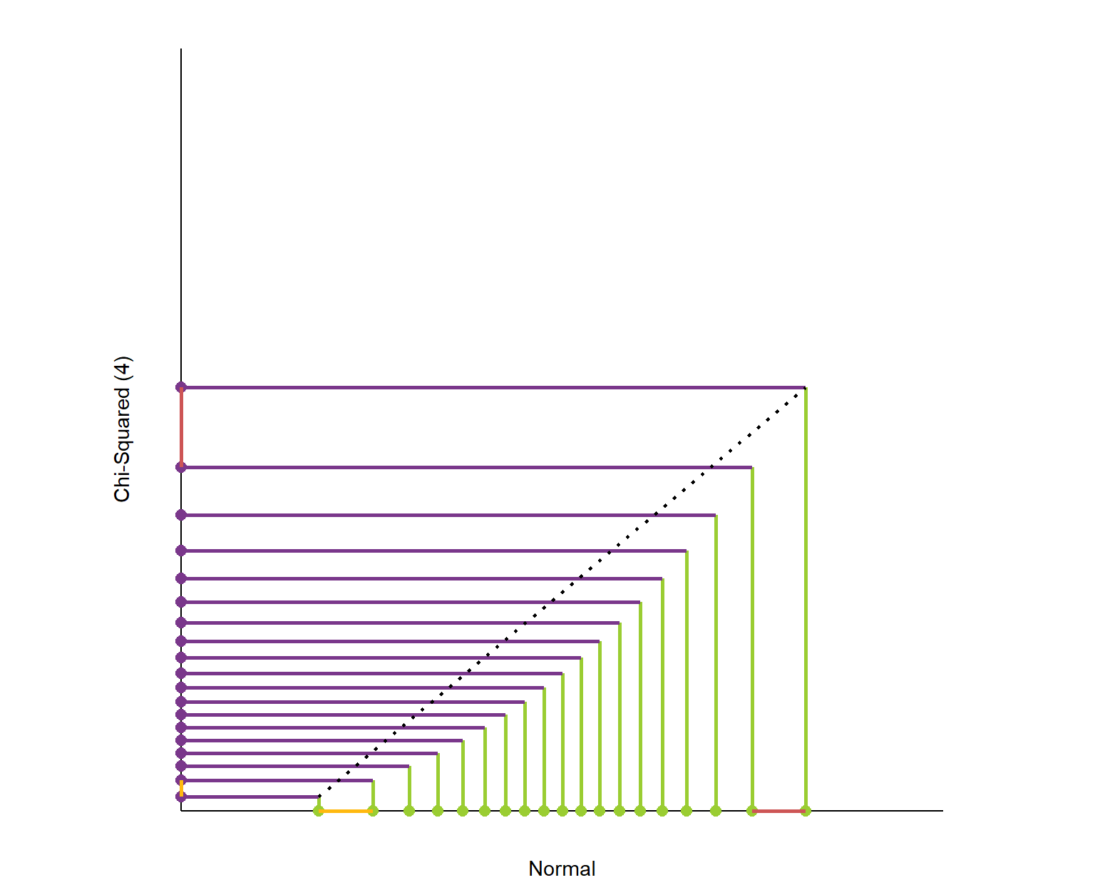
A receiver operating characteristic (ROC) curve displays how well a model can classify binary outcomes. An ROC curve is generated by plotting the false positive rate of a model against its true positive rate, for each possible cutoff value. Often, the area under the curve (AUC) is calculated and used as a metric showing how well a model can classify data points.

If you’re interest in learning more about ROC and AUC, I recommend this short Medium blog, which contains this neat graphic:

Dariya Sydykova, graduate student at the Wilke lab at the University of Texas at Austin, shared some great visual animations of how model accuracy and model cutoffs alter the ROC curve and the AUC metric. The quotes and animations are from the associated github repository.

ROC & AUC

The plot on the left shows the distributions of predictors for the two outcomes, and the plot on the right shows the ROC curve for these distributions. The vertical line that travels left-to-right is the cutoff value. The red dot that travels along the ROC curve corresponds to the false positive rate and the true positive rate for the cutoff value given in the plot on the left.
The traveling cutoff demonstrates the trade-off between trying to classify one outcome correctly and trying to classify the other outcome correcly. When we try to increase the true positive rate, we also increase the false positive rate. When we try to decrease the false positive rate, we decrease the true positive rate.

The shape of an ROC curve changes when a model changes the way it classifies the two outcomes.
The animation [below] starts with a model that cannot tell one outcome from the other, and the two distributions completely overlap (essentially a random classifier). As the two distributions separate, the ROC curve approaches the left-top corner, and the AUC value of the curve increases. When the model can perfectly separate the two outcomes, the ROC curve forms a right angle and the AUC becomes 1.

Precision-Recall

Two other metrics that are often used to quantify model performance are precision and recall.

Precision (also called positive predictive value) is defined as the number of true positives divided by the total number of positive predictions. Hence, precision quantifies what percentage of the positive predictions were correct: How correct your model’s positive predictions were.

Recall (also called sensitivity) is defined as the number of true positives divided by the total number of true postives and false negatives (i.e. all actual positives). Hence, recall quantifies what percentage of the actual positives you were able to identify: How sensitive your model was in identifying positives.

Dariya also made some visualizations of precision-recall curves:

Precision-recall curves also displays how well a model can classify binary outcomes. However, it does it differently from the way an ROC curve does. Precision-recall curve plots true positive rate (recall or sensitivity) against the positive predictive value (precision).

In the middle, here below, the ROC curve with AUC. On the right, the associated precision-recall curve.

Similarly to the ROC curve, when the two outcomes separate, precision-recall curves will approach the top-right corner. Typically, a model that produces a precision-recall curve that is closer to the top-right corner is better than a model that produces a precision-recall curve that is skewed towards the bottom of the plot.

Class imbalance

Class imbalance happens when the number of outputs in one class is different from the number of outputs in another class. For example, one of the distributions has 1000 observations and the other has 10. An ROC curve tends to be more robust to class imbalanace that a precision-recall curve.
In this animation [below], both distributions start with 1000 outcomes. The blue one is then reduced to 50. The precision-recall curve changes shape more drastically than the ROC curve, and the AUC value mostly stays the same. We also observe this behaviour when the other disribution is reduced to 50.

Here’s the same, but now with the red distribution shrinking to just 50 samples.

Dariya invites you to use these visualizations for educational purposes:

Please feel free to use the animations and scripts in this repository for teaching or learning. You can directly download the gif files for any of the animations, or you can recreate them using these scripts. Each script is named according to the animation it generates (i.e. animate_ROC.r generates ROC.gif, animate_SD.r generates SD.gif, etc.).

Want to learn more about the different evaluation metrics for machine learning? Here’s a nice how-to guide by Neptune.ai demonstrating different metrics applied in Python.

Understanding Data Distributions

Having trouble understanding how to interpret distribution plots? Or struggling with Q-Q plots? Sven Halvorson penned down a visual tutorial explaining distributions using visualisations of their quantiles.

Because each slice of the distribution is 5% of the total area and the height of the graph is changing, the slices have different widths. It’s like we’re trying to cut a strange shaped cake into 20 equal pieces using parallel cuts. The slices at the center must be thinner since the distribution is denser (taller) than on the edges.
Sven on distribution signatures

Here is the plot of matching the quantiles of the chi-squared(4) and normal distributions. I’ve again plotted these quantiles over 98% of each distribution’s range. The chi-squared distribution is skewed so its quantiles are packed into a smaller portion of its axis.

What is this graph telling us? It shows that the exchange rate between the quantiles of the two distributions is not constant.
Sven on distribution signatures

Here’s the link to the original article, and the R markdown code on github to generate the webpage.

Two Tinder Experiments: An Unequal Economy

I’ve seen a fair share of Tinder experiments come by, for instance, someone A/B-testing attractiveness with and without facial hair, but these new two posts on Medium are the best I’ve come across so far.

In his first experiment, this self-proclaimed worst online dater went catfishing. He made a Tinder account using stock photos of attractive and less attractive and old and young guys, looking and sampled some like ratio’s.

Basically, his conclusion was that “Tinder actually can work, but pretty much only if you are an attractive guy”

The statistics of the first experiment:
https://worst-online-dater.tumblr.com/post/99441021279/tinder-experiments

In the second experiment, the author decided to treat Tinder as an economy and study it as an (socio-)economist would:

The wealth of an economy is quantified in terms its currency. […] In Tinder the currency is “likes”. […] Wealth in Tinder is not distributed equally. Attractive guys have more wealth in the Tinder economy (get more “likes”) than unattractive guys do. […] An unequal wealth distribution is to be expected, but there is a more interesting question: What is the degree of this unequal wealth distribution and how does this inequality compare to other economies?
Original Medium Post by Worst Online Dater

The author notes some caveats of this analysis. First and foremost, the data was collected in quite an unethical way, by asking questions to 27 of the matches with the fake accounts the author set up. Moreover, self-report bias is quite likely, as it’s easy to lie on Tinder. Still, the results are quite amusing:

Basically, “the bottom 80% of men are fighting over the bottom 22% of women and the top 78% of women are fighting over the top 20% of men”

The Lorenz curve shows the proportion of wealth owned by the bottom x% of a population. If wealth was equally distributed the curve would be perfectly diagonal (a 45 degree slope). The steeper the slope, the less inequal an economy. The below shows the curve for a perfectly equal economy, the US economy, and the estimated Tinder economy:

Similarly, the Gini coefficient can be used to represent the wealth equality of an economy. It ranges from 0 to 1, where 0 corresponds with perfect equality (everybody has the same wealth) and 1 corresponds with perfect inequality (one dictator with all the wealth). While most European countries, and even the US, score quite low on this Gini index, the Tinder economy is estimated to be much more towards the lower end.

Finally, based on the collected data, the author was able to reduce Tinder Male Attractiveness to a function of the number of likes received:

According to my last post, the most attractive men will be liked by only approximately 20% of all the females on Tinder. […] Unfortunately, this percentage decreases rapidly as you go down the attractiveness scale. According to this analysis a man of average attractiveness can only expect to be liked by slightly less than 1% of females (0.87%). This equates to 1 “like” for every 115 females.
The good news is that if you are only getting liked by a few girls on Tinder you shouldn’t take it personally. You aren’t necessarily unattractive. You can be of above average attractiveness and still only get liked by a few percent of women on Tinder. The bad news is that if you aren’t in the very upper echelons of Tinder wealth (i.e. attractiveness) you aren’t likely to have much success using Tinder. You would probably be better off just going to a bar or joining some coed recreational sports team.
Original Medium Post by Worst Online Dater

E-Book: Probabilistic Programming & Bayesian Methods for Hackers

The Bayesian method is the natural approach to inference, yet it is hidden from readers behind chapters of slow, mathematical analysis. Nevertheless, mathematical analysis is only one way to “think Bayes”. With cheap computing power, we can now afford to take an alternate route via probabilistic programming.

Cam Davidson-Pilon wrote the book Bayesian Methods for Hackers as a introduction to Bayesian inference from a computational and understanding-first, mathematics-second, point of view.

The book is available via Amazon, but you can access an online e-book for free. There’s also an associated GitHub repo.

The book explains Bayesian principles with code and visuals. For instance:

%matplotlib inline
from IPython.core.pylabtools import figsize
import numpy as np
from matplotlib import pyplot as plt
figsize(11, 9)

import scipy.stats as stats

dist = stats.beta
n_trials = [0, 1, 2, 3, 4, 5, 8, 15, 50, 500]
data = stats.bernoulli.rvs(0.5, size=n_trials[-1])
x = np.linspace(0, 1, 100)

for k, N in enumerate(n_trials):
    sx = plt.subplot(len(n_trials)/2, 2, k+1)
    plt.xlabel("$p$, probability of heads") \
        if k in [0, len(n_trials)-1] else None
    plt.setp(sx.get_yticklabels(), visible=False)
    heads = data[:N].sum()
    y = dist.pdf(x, 1 + heads, 1 + N - heads)
    plt.plot(x, y, label="observe %d tosses,\n %d heads" % (N, heads))
    plt.fill_between(x, 0, y, color="#348ABD", alpha=0.4)
    plt.vlines(0.5, 0, 4, color="k", linestyles="--", lw=1)

    leg = plt.legend()
    leg.get_frame().set_alpha(0.4)
    plt.autoscale(tight=True)


plt.suptitle("Bayesian updating of posterior probabilities",
             y=1.02,
             fontsize=14)

plt.tight_layout()

I can only recommend you start with the online version of Bayesian Methods for Hackers, but note that the print version helps sponsor the author ánd includes some additional features:

Additional Chapter on Bayesian A/B testing
Updated examples
Answers to the end of chapter questions
Additional explanation, and rewritten sections to aid the reader.

If you’re interested in learning more about Bayesian analysis, I recommend these other books:

Northstar: The interactive, drag-and-drop data science platform by MIT

MIT researchers have spent years developing the new drag-and-drop analytics tools they call Northstar.

Northstar is an interactive data science platform that rethinks how people interact with data. It empowers users without programming experience, background in statistics or machine learning expertise to explore and mine data through an intuitive user interface, and effortlessly build, analyze, and evaluate machine learning (ML) pipelines.
northstar.mit.edu/

Northstar starts as a blank, white interface. Users upload datasets into the system, which appear in a “datasets” box on the left. Any data labels will automatically populate a separate “attributes” box below. There’s also an “operators” box that contains various algorithms, as well as the new AutoML tool. All data are stored and analyzed in the cloud.
news.mit.edu/2019/drag-drop-data-analytics-0627

You can read more about the tool’s functionalities in this MIT news article, which includes several promising GIFs:

Moreover, on the Northstar website you can find this longer video explaining the tool in detail.

https://vimeo.com/342787403

While Northstar looks insanely cool and promising, I do worry about putting such power in the hands of people who may not have much experience with statistics and/or machine learning. We all know how easily errors and bias may slip into data-driven processes, so I am curious to see how these next-gen kind of tools will be deployed and used.

Generalized Additive Models Tutorial in R, by Noam Ross

Generalized Additive Models — or GAMs in short — have been somewhat of a mystery to me. I’ve known about them, but didn’t know exactly what they did, or when they’re useful. That came to an end when I found out about this tutorial by Noam Ross.

In this beautiful, online, interactive course, Noam allows you to program several GAMs yourself (in R) and to progressively learn about the different functions and features. I am currently halfway through, but already very much enjoy it.

If you’re already familiar with linear models and want to learn something new, I strongly recommend this course!