Tag: academia

Create a publication-ready correlation matrix, with significance levels, in R

Create a publication-ready correlation matrix, with significance levels, in R

TLDR; You can use the corrtable package (see CRAN or Github)!

In most (observational) research papers you read, you will probably run into a correlation matrix. Often it looks something like this:

FACTOR ANALYSIS

In Social Sciences, like Psychology, researchers like to denote the statistical significance levels of the correlation coefficients, often using asterisks (i.e., *). Then the table will look more like this:

Table 4 from Family moderators of relation between community ...

Regardless of my personal preferences and opinions, I had to make many of these tables for the scientific (non-)publications of my Ph.D..

I remember that, when I first started using R, I found it quite difficult to generate these correlation matrices automatically.

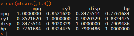
Yes, there is the cor function, but it does not include significance levels.

Then there the (in)famous Hmisc package, with its rcorr function. But this tool provides a whole new range of issues.

What’s this storage.mode, and what are we trying to coerce again?

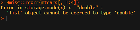
Soon you figure out that Hmisc::rcorr only takes in matrices (thus with only numeric values). Hurray, now you can run a correlation analysis on your dataframe, you think…

Yet, the output is all but publication-ready!

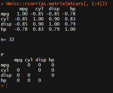
You wanted one correlation matrix, but now you have two… Double the trouble?

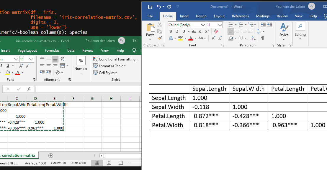
[UPDATED] To spare future scholars the struggle of the early day R programming, Laura Lambert and I created an R package corrtable, which includes the helpful function correlation_matrix.

This correlation_matrix takes in a dataframe, selects only the numeric (and boolean/logical) columns, calculates the correlation coefficients and p-values, and outputs a fully formatted publication-ready correlation matrix!

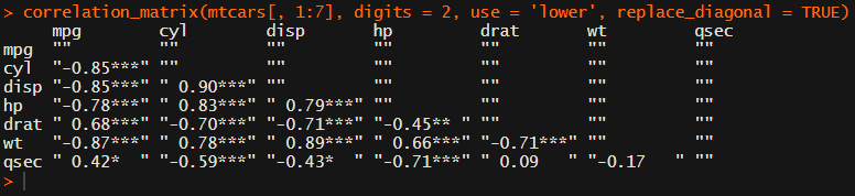
You can specify many formatting options in correlation_matrix.

For instance, you can use only 2 decimals. You can focus on the lower triangle (as the lower and upper triangle values are identical). And you can drop the diagonal values:

Or maybe you are interested in a different type of correlation coefficients, and not so much in significance levels:

For other formatting options, do have a look at the source code on github.

Now, to make matters even easier, the package includes a second function (save_correlation_matrix) to directly save any created correlation matrices:

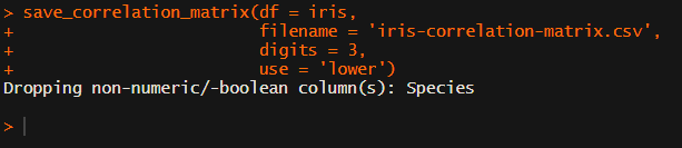
Once you open your new correlation matrix file in Excel, it is immediately ready to be copy-pasted into Word!

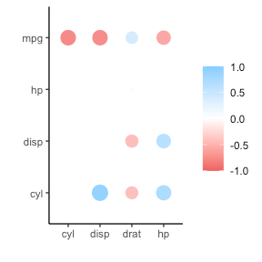
If you are looking for ways to visualize your correlations do have a look at the packages corrr, corrplot, or ppsr.

I hope this package is of help to you!

Do reach out if you get to use them in any of your research papers!

Sign up to keep up to date on the latest R, Data Science & Tech content:

Anomaly Detection Resources

Anomaly Detection Resources

Carnegie Mellon PhD student Yue Zhao collects this great Github repository of anomaly detection resources: https://github.com/yzhao062/anomaly-detection-resources

The repository consists of tools for multiple languages (R, Python, Matlab, Java) and resources in the form of:

  1. Books & Academic Papers
  2. Online Courses and Videos
  3. Outlier Datasets
  4. Algorithms and Applications
  5. Open-source and Commercial Libraries/Toolkits
  6. Key Conferences & Journals

Outlier Detection (also known as Anomaly Detection) is an exciting yet challenging field, which aims to identify outlying objects that are deviant from the general data distribution. Outlier detection has been proven critical in many fields, such as credit card fraud analytics, network intrusion detection, and mechanical unit defect detection.

https://github.com/yzhao062/anomaly-detection-resources

Quick Access — Table of Contents

ggstatsplot: Creating graphics including statistical details

ggstatsplot: Creating graphics including statistical details

This pearl had been resting in my inbox for quite a while before I was able to add it to my R resources list. Citing its GitHub pageggstatsplot is an extension of ggplot2 package for creating graphics with details from statistical tests included in the plots themselves and targeted primarily at behavioral sciences community to provide a one-line code to produce information-rich plots. The package is currently maintained and still under development by Indrajeet Patil. Nevertheless, its functionality is already quite impressive. You can download the latest stable version via:

utils::install.packages(pkgs = "ggstatsplot")

Or download the development version via:

devtools::install_github(
  repo = "IndrajeetPatil/ggstatsplot", # package path on GitHub
  dependencies = TRUE,                 # installs packages which ggstatsplot depends on
  upgrade_dependencies = TRUE          # updates any out of date dependencies
)

The package currently supports many different statistical plots, including:

?ggbetweenstats
?ggscatterstats
?gghistostats
?ggpiestats
?ggcorrmat
?ggcoefstats
?combine_plots
?grouped_ggbetweenstats
?grouped_ggscatterstats
?grouped_gghistostats
?grouped_ggpiestats
?grouped_ggcorrmat

Let’s take a closer look at the first one:

ggbetweenstats

This function creates either a violin plot, a box plot, or a mix of two for between-group or between-condition comparisons and additional detailed results from statistical tests can be added in the subtitle. The simplest function call looks like the below, but much more complex information can be added and specified.

set.seed(123) # to get reproducible results

# the functions work approximately the same as ggplot2
ggstatsplot::ggbetweenstats(
  data = datasets::iris, 
  x = Species, 
  y = Sepal.Length,
  messages = FALSE
) +   
# and can be adjusted using the same, orginal function calls
  ggplot2::coord_cartesian(ylim = c(3, 8)) + 
  ggplot2::scale_y_continuous(breaks = seq(3, 8, by = 1))

All pictures copied from the GitHub page of ggstatsplot [original]

ggscatterstats

Not all plots are ggplot2-compatible though, for instance, ggscatterstats is not. Nevertheless, it produces a very powerful plot in my opinion.

ggstatsplot::ggscatterstats(
  data = datasets::iris, 
  x = Sepal.Length, 
  y = Petal.Length,
  title = "Dataset: Iris flower data set",
  messages = FALSE
)

All pictures copied from the GitHub page of ggstatsplot [original]

ggcormat

ggcorrmat is also quite impressive, producing correlalograms with only minimal amounts of code as it wraps around ggcorplot. The defaults already produces publication-ready correlation matrices:

ggstatsplot::ggcorrmat(
  data = datasets::iris,
  corr.method = "spearman",
  sig.level = 0.005,
  cor.vars = Sepal.Length:Petal.Width,
  cor.vars.names = c("Sepal Length", "Sepal Width", "Petal Length", "Petal Width"),
  title = "Correlalogram for length measures for Iris species",
  subtitle = "Iris dataset by Anderson",
  caption = expression(
    paste(
      italic("Note"),
      ": X denotes correlation non-significant at ",
      italic("p "),
      "< 0.005; adjusted alpha"
    )
  )
)

All pictures copied from the GitHub page of ggstatsplot [original]

ggcoefstats

Finally, ggcoefstats is a wrapper around GGally::ggcoef, creating a plot with the regression coefficients’ point estimates as dots with confidence interval whiskers. Here’s an example with some detailed specifications:

ggstatsplot::ggcoefstats(
  x = stats::lm(formula = mpg ~ am * cyl,
                data = datasets::mtcars),
  point.color = "red",
  vline.color = "#CC79A7",
  vline.linetype = "dotdash",
  stats.label.size = 3.5,
  stats.label.color = c("#0072B2", "#D55E00", "darkgreen"),
  title = "Car performance predicted by transmission and cylinder count",
  subtitle = "Source: 1974 Motor Trend US magazine"
) +                                    
  ggplot2::scale_y_discrete(labels = c("transmission", "cylinders", "interaction")) +
  ggplot2::labs(x = "regression coefficient",
                y = NULL)

All pictures copied from the GitHub page of ggstatsplot [original]
I for one am very curious to see how Indrajeet will further develop this package, and whether academics will start using it as a default in publishing.


Network Visualization with igraph and ggraph

Network Visualization with igraph and ggraph

Eiko Fried, researcher at the University of Amsterdam, recently blogged about personal collaborator networks. I came across his post on twitter, discussing how to conduct such analysis in R, and got inspired.

Unfortunately, my own publication record is quite boring to analyse, containing only a handful of papers. However, my promotors – Prof. dr. Jaap Paauwe and Prof. dr. Marc van Veldhoven – have more extensive publication lists. Although I did not manage to retrieve those using the scholarpackage, I was able to scrape Jaap Paauwe’s publication list from his Google Scholar page. Jaap has 141 publications listed with one or more citation on Google Scholar. More than enough for an analysis!

While Eiko uses his colleague Sacha Epskamp’s R package qgraph, I found an alternative in the packages igraph and ggraph.

### PAUL VAN DER LAKEN
### 2017-10-31
### COAUTHORSHIP NETWORK VISUALIZATION

# LOAD IN PACKAGES
library(readxl)
library(dplyr)
library(ggraph)
library(igraph)

# STANDARDIZE VISUALIZATIONS
w = 14
h = 7
dpi = 900

# LOAD IN DATA
pub_history <- read_excel("paauwe_wos.xlsx")

# RETRIEVE AUTHORS
pub_history %>%
  filter(condition == 1) %>%
  select(name) %>%
  .$name %>%
  gsub("[A-Z]{2,}|[A-Z][ ]", "", .) %>%
  strsplit(",") %>%
  lapply(function(x) gsub("\\..*", "", x)) %>%
  lapply(function(x) gsub("^[ ]+","",x)) %>%
  lapply(function(x) x[x != ""]) %>%
  lapply(function(x) tolower(x))->
  authors

# ADD JAAP PAAUWE WHERE MISSING
authors <- lapply(authors, function(x){
  if(!"paauwe" %in% x){
    return(c(x,"paauwe"))
  } else{
    return(x)
  }
})

# EXTRACT UNIQUE AUTHORS
authors_unique <- authors %>% unlist() %>% unique() %>% sort(F)

# FORMAT AUTHOR NAMES 
# CAPATILIZE
simpleCap <- function(x) {
  s <- strsplit(x, " ")[[1]]
  names(s) <- NULL
  paste(toupper(substring(s, 1,1)), substring(s, 2),
        sep="", collapse=" ")
}
authors_unique_names <- sapply(authors_unique, simpleCap)

The above retrieve the names of every unique author from the excel file I got from Google Scholar. Now we need to examine to what extent the author names co-occur. We do that with the below code, storing all co-occurance data in a matrix, which we then transform to an adjacency matrix igraph can deal with. The output graph data looks like this:

# CREATE COAUTHORSHIP MATRIX
coauthorMatrix <- do.call(
  cbind,
  lapply(authors, function(x){
  1*(authors_unique %in% x)
}))

# TRANSFORM TO ADJECENY MATRIX
adjacencyMatrix <- coauthorMatrix %*% t(coauthorMatrix)

# CREATE NETWORK GRAPH
g <- graph.adjacency(adjacencyMatrix, 
                     mode = "undirected", 
                     diag = FALSE)
V(g)$Degree <- degree(g, mode = 'in') # CALCULATE DEGREE
V(g)$Name <- authors_unique_names # ADD NAMES
g # print network
## IGRAPH f1b50a7 U--- 168 631 -- 
## + attr: Degree (v/n), Name (v/c)
## + edges from f1b50a7:
##  [1]  1-- 21  1--106  2-- 44  2-- 52  2--106  2--110  3-- 73  3--106
##  [9]  4-- 43  4-- 61  4-- 78  4-- 84  4--106  5-- 42  5--106  6-- 42
## [17]  6-- 42  6-- 97  6-- 97  6--106  6--106  6--125  6--125  6--127
## [25]  6--127  6--129  6--129  7--106  7--106  7--150  7--150  8-- 24
## [33]  8-- 38  8-- 79  8-- 98  8-- 99  8--106  9-- 88  9--106  9--133
## [41] 10-- 57 10--106 10--128 11-- 76 11-- 85 11--106 12-- 30 12-- 80
## [49] 12--106 12--142 12--163 13-- 16 13-- 16 13-- 22 13-- 36 13-- 36
## [57] 13--106 13--106 13--106 13--166 14-- 70 14-- 94 14--106 14--114
## + ... omitted several edges

This graph data we can now feed into ggraph:

# SET THEME FOR NETWORK VISUALIZATION
theme_networkMap <- theme(
  plot.background = element_rect(fill = "beige"),
  panel.border = element_blank(),
  panel.grid = element_blank(),
  panel.background = element_blank(),
  legend.background = element_blank(),
  legend.position = "none",
  legend.title = element_text(colour = "black"),
  legend.text = element_text(colour = "black"),
  legend.key = element_blank(),
  axis.text = element_blank(), 
  axis.title = element_blank(),
  axis.ticks = element_blank()
)
# VISUALIZE NETWORK
ggraph(g, layout = "auto") +
  # geom_edge_density() +
  geom_edge_diagonal(alpha = 1, label_colour = "blue") +
  geom_node_label(aes(label = Name, size = sqrt(Degree), fill = sqrt(Degree))) +
  theme_networkMap +
  scale_fill_gradient(high = "blue", low = "lightblue") +
  labs(title = "Coauthorship Network of Jaap Paauwe",
       subtitle = "Publications with more than one Google Scholar citation included",
       caption = "paulvanderlaken.com") +
  ggsave("Paauwe_Coauthorship_Network.png", dpi = dpi, width = w, height = h)

Paauwe_Coauthorship_Network

Feel free to use the code to look at your own coauthorship networks or to share this further.