Tag: correlation

ppsr: An R implementation of the Predictive Power Score

ppsr: An R implementation of the Predictive Power Score

Update March, 2021: My R package for the predictive power score (ppsr) is live on CRAN!
Try install.packages("ppsr") in your R terminal to get the latest version.

A few months ago, I wrote about the Predictive Power Score (PPS): a handy metric to quickly explore and quantify the relationships in a dataset.

As a social scientist, I was taught to use a correlation matrix to describe the relationships in a dataset. Yet, in my opinion, the PPS provides three handy advantages:

  1. PPS works for any type of data, also nominal/categorical variables
  2. PPS quantifies non-linear relationships between variables
  3. PPS acknowledges the asymmetry of those relationships

Florian Wetschoreck came up with the PPS idea, wrote the original blog, and programmed a Python implementation of it (called ppscore).

Yet, I work mostly in R and I was very keen on incorporating this powertool into my general data science workflow.

So, over the holiday period, I did something I have never done before: I wrote an R package!

It’s called ppsr and you can find the code here on github.

Installation

# You can get the official version from CRAN:
install.packages("ppsr")

## Or you can get the development version from GitHub:
# install.packages('devtools')
# devtools::install_github('https://github.com/paulvanderlaken/ppsr')

Usage

The ppsr package has three main functions that compute PPS:

  • score() – which computes an x-y PPS
  • score_predictors() – which computes X-y PPS
  • score_matrix() – which computes X-Y PPS

Visualizing PPS

Subsequently, there are two main functions that wrap around these computational functions to help you visualize your PPS using ggplot2:

  • visualize_predictors() – producing a barplot of all X-y PPS
  • visualize_matrix() – producing a heatmap of all X-Y PPS
PPS matrix for iris

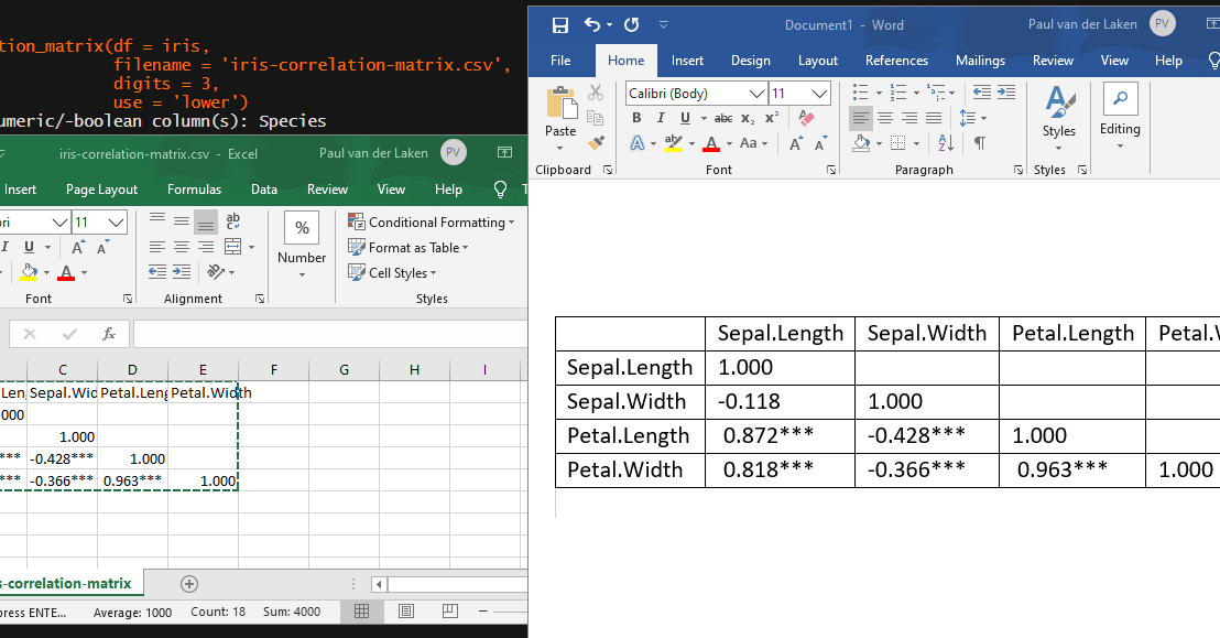
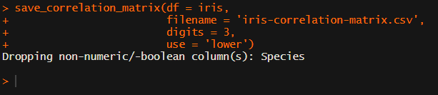
Note that Species is a nominal/categorical variable, with three character/text options.

A correlation matrix would not be able to show us that the type of iris Species can be predicted extremely well by the petal length and width, and somewhat by the sepal length and width. Yet, particularly sepal width is not easily predicted by the type of species.
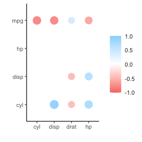
Correlation matrix for iris

Exploring mtcars

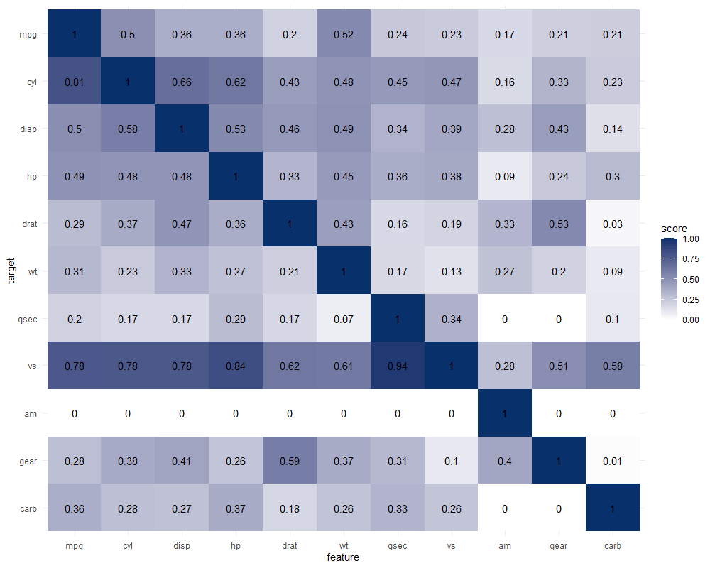
It takes about 10 seconds to run 121 decision trees with visualize_matrix(mtcars). Yet, the output is much more informative than the correlation matrix:

  • cyl can be much better predicted by mpg than the other way around
  • the classification of vs can be done well using nearly all variables as predictors, except for am
  • yet, it’s hard to predict anything based on the vs classification
  • a cars’ am can’t be predicted at all using these variables
PPS matrix for mtcars

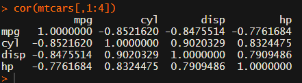
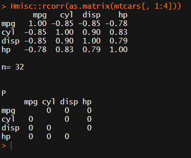
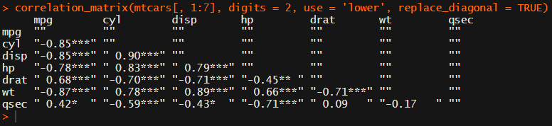
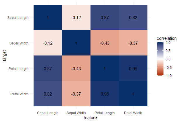
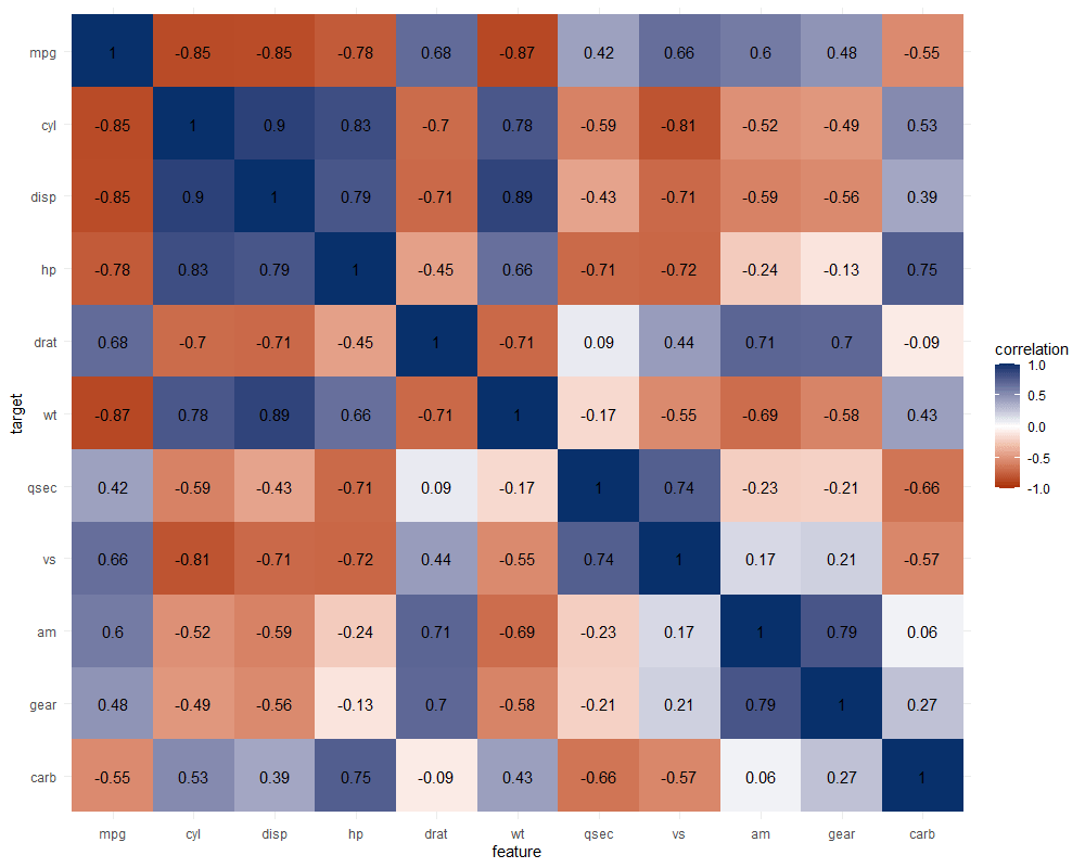
The correlation matrix does provides insights that are not provided by the PPS matrix. Most importantly, the sign and strength of any linear relationship that may exist. For instance, we can deduce that mpg relates strongly negatively with cyl.

Yet, even though half of the matrix does not provide any additional information (due to the symmetry), I still find it hard to derive the most important relations and insights at a first glance.

Moreover, the rows and columns for vs and am are not very informative in this correlation matrix as it contains pearson correlations coefficients by default, whereas vs and am are binary variables. The same can be said for cyl, gear and carb, which contain ordinal categories / integer data, so you can discuss the value of these coefficients depicted here.

Correlation matrix for mtcars

Exploring trees

In R, there are many datasets built in via the datasets package. Let’s explore some using the ppsr::visualize_matrix() function.

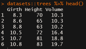
datasets::trees has data on 31 trees’ girth, height and volume.

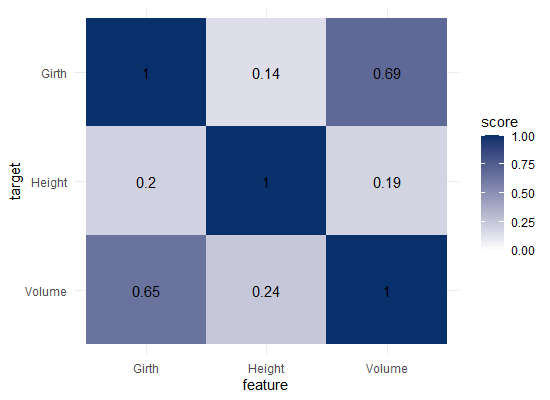
visualize_matrix(datasets::trees) shows that both girth and volume can be used to predict the other quite well, but not perfectly.

Let’s have a look at the correlation matrix.

The scores here seem quite higher in general. A near perfect correlation between volume and girth.

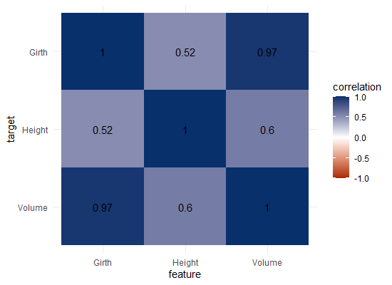
Is it near perfect though? Let’s have a look at the underlying data and fit a linear model to it.

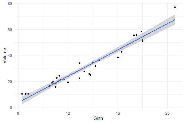
You will still be pretty far off the real values when you use a linear model based on Girth to predict Volume. This is what the original PPS of 0.65 tried to convey.

Actually, I’ve run the math for this linaer model and the RMSE is still 4.11. Using just the mean Volume as a prediction of Volume will result in 16.17 RMSE. If we map these RMSE values on a linear scale from 0 to 1, we would get the PPS of our linear model, which is about 0.75.

So, actually, the linear model is a better predictor than the decision tree that is used as a default in the ppsr package. That was used to generate the PPS matrix above.

Yet, the linear model definitely does not provide a perfect prediction, even though the correlation may be near perfect.

Conclusion

In sum, I feel using the general idea behind PPS can be very useful for data exploration.

Particularly in more data science / machine learning type of projects. The PPS can provide a quick survey of which targets can be predicted using which features, potentially with more complex than just linear patterns.

Yet, the old-school correlation matrix also still provides unique and valuable insights that the PPS matrix does not. So I do not consider the PPS so much an alternative, as much as a complement in the toolkit of the data scientist & researcher.

Enjoy the R package, or the Python module for that matter, and let me know if you see any improvements!

How most statistical tests are linear models

How most statistical tests are linear models

Jonas Kristoffer Lindeløv wrote a great visual explanation of how the most common statistical tests (t-test, ANOVA, ANCOVA, etc) are all linear models in the back-end.

Jonas’ original blog uses R programming to visually show how the tests work, what the linear models look like, and how different approaches result in the same statistics.

George Ho later remade a Python programming version of the same visual explanation.

If I was thought statistics and methodology this way, I sure would have struggled less! Have a look yourself: https://lindeloev.github.io/tests-as-linear/

Create a publication-ready correlation matrix, with significance levels, in R

Create a publication-ready correlation matrix, with significance levels, in R

TLDR; You can use the corrtable package (see CRAN or Github)!

In most (observational) research papers you read, you will probably run into a correlation matrix. Often it looks something like this:

FACTOR ANALYSIS

In Social Sciences, like Psychology, researchers like to denote the statistical significance levels of the correlation coefficients, often using asterisks (i.e., *). Then the table will look more like this:

Table 4 from Family moderators of relation between community ...

Regardless of my personal preferences and opinions, I had to make many of these tables for the scientific (non-)publications of my Ph.D..

I remember that, when I first started using R, I found it quite difficult to generate these correlation matrices automatically.

Yes, there is the cor function, but it does not include significance levels.

Then there the (in)famous Hmisc package, with its rcorr function. But this tool provides a whole new range of issues.

What’s this storage.mode, and what are we trying to coerce again?

Soon you figure out that Hmisc::rcorr only takes in matrices (thus with only numeric values). Hurray, now you can run a correlation analysis on your dataframe, you think…

Yet, the output is all but publication-ready!

You wanted one correlation matrix, but now you have two… Double the trouble?

[UPDATED] To spare future scholars the struggle of the early day R programming, Laura Lambert and I created an R package corrtable, which includes the helpful function correlation_matrix.

This correlation_matrix takes in a dataframe, selects only the numeric (and boolean/logical) columns, calculates the correlation coefficients and p-values, and outputs a fully formatted publication-ready correlation matrix!

You can specify many formatting options in correlation_matrix.

For instance, you can use only 2 decimals. You can focus on the lower triangle (as the lower and upper triangle values are identical). And you can drop the diagonal values:

Or maybe you are interested in a different type of correlation coefficients, and not so much in significance levels:

For other formatting options, do have a look at the source code on github.

Now, to make matters even easier, the package includes a second function (save_correlation_matrix) to directly save any created correlation matrices:

Once you open your new correlation matrix file in Excel, it is immediately ready to be copy-pasted into Word!

If you are looking for ways to visualize your correlations do have a look at the packages corrr, corrplot, or ppsr.

I hope this package is of help to you!

Do reach out if you get to use them in any of your research papers!

Sign up to keep up to date on the latest R, Data Science & Tech content:

Predictive Power Score: Finding predictive patterns in your dataset

Predictive Power Score: Finding predictive patterns in your dataset

Update March, 2021: My R package for the predictive power score (ppsr) is live on CRAN!
Try install.packages("ppsr") in your R terminal to get the latest version.

Last week, I shared this Medium blog on PPS — or Predictive Power Score — on my LinkedIn and got so many enthousiastic responses, that I had to share it with here too.

Basically, the predictive power score is a normalized metric (values range from 0 to 1) that shows you to what extent you can use a variable X (say age) to predict a variable Y (say weight in kgs).

A PPS high score of, for instance, 0.85, would show that weight can be predicted pretty good using age.

A low PPS score, of say 0.10, would imply that weight is hard to predict using age.

The PPS acts a bit like a correlation coefficient we’re used too, but it is also different in many ways that are useful to data scientists:

  1. PPS also detects and summarizes non-linear relationships
  2. PPS is assymetric, so that it models Y ~ X, but not necessarily X ~ Y
  3. PPS can summarize predictive value of / among categorical variables and nominal data

However, you may argue that the PPS is harder to interpret than the common correlation coefficent:

  1. PPS can reflect quite complex and very different patterns
  2. Therefore, PPS are hard to compare: a 0.5 may reflect a linear relationship but also many other relationships
  3. PPS are highly dependent on the used algorithm: you can use any algorithm from OLS to CART to full-blown NN or XGBoost. Your algorithm hihgly depends the patterns you’ll detect and thus your scores
  4. PPS are highly dependent on the the evaluation metric (RMSE, MAE, etc).

Here’s an example picture from the original blog, showing a case in which PSS shows the relevant predictive value of Y ~ X, whereas a correlation coefficient would show no relationship whatsoever:

https://towardsdatascience.com/rip-correlation-introducing-the-predictive-power-score-3d90808b9598

Here’s two more pictures from the original blog showing the differences with a standard correlation matrix on the Titanic data:

I highly suggest you read the original blog for more details and information, and that you check out the associated Python package ppscore:

Installing the package:

pip install ppscore

Calculating the PPS for a given pandas dataframe:

import ppscore as pps
pps.score(df, "feature_column", "target_column")

You can also calculate the whole PPS matrix:

pps.matrix(df)

There’s no R package yet, but it should not be hard to implement this general logic.

Florian Wetschoreck — the author — already noted that there may be several use cases where he’d think PPS may add value:

Find patterns in the data [red: data exploration]: The PPS finds every relationship that the correlation finds — and more. Thus, you can use the PPS matrix as an alternative to the correlation matrix to detect and understand linear or nonlinear patterns in your data. This is possible across data types using a single score that always ranges from 0 to 1.

Feature selection: In addition to your usual feature selection mechanism, you can use the predictive power score to find good predictors for your target column. Also, you can eliminate features that just add random noise. Those features sometimes still score high in feature importance metrics. In addition, you can eliminate features that can be predicted by other features because they don’t add new information. Besides, you can identify pairs of mutually predictive features in the PPS matrix — this includes strongly correlated features but will also detect non-linear relationships.

Detect information leakage: Use the PPS matrix to detect information leakage between variables — even if the information leakage is mediated via other variables.

Data Normalization: Find entity structures in the data via interpreting the PPS matrix as a directed graph. This might be surprising when the data contains latent structures that were previously unknown. For example: the TicketID in the Titanic dataset is often an indicator for a family.

https://towardsdatascience.com/rip-correlation-introducing-the-predictive-power-score-3d90808b9598
18 Pitfalls of Data Visualization

18 Pitfalls of Data Visualization

Maarten Lambrechts is a data journalist I closely follow online, with great delight. Recently, he shared on Twitter his slidedeck on the 18 most common data visualization pitfalls. You will probably already be familiar with most, but some (like #14) were new to me:

  1. Save pies for dessert
  2. Don’t cut bars
  3. Don’t cut time axes
  4. Label directly
  5. Use colors deliberately
  6. Avoid chart junk
  7. Scale circles by area
  8. Avoid double axes
  9. Correlation is no causality
  10. Don’t do 3D
  11. Sort on the data
  12. Tell the story
  13. 1 chart, 1 message
  14. Common scales on small mult’s
  15. #Endrainbow
  16. Normalise data on maps
  17. Sometimes best map is no map
  18. All maps lie

Even though most of these 18 rules below seem quite obvious, even the European Commissions seems to break them every now and then:

Can you spot what’s wrong with this graph?

Simple Correlation Analysis in R using Tidyverse Principles

Simple Correlation Analysis in R using Tidyverse Principles

R’s standard correlation functionality (base::cor) seems very impractical to the new programmer: it returns a matrix and has some pretty shitty defaults it seems. Simon Jackson thought the same so he wrote a tidyverse-compatible new package: corrr!

Simon wrote some practical R code that has helped me out greatly before (e.g., color palette’s), but this new package is just great. He provides an elaborate walkthrough on his own blog, which I can highly recommend, but I copied some teasers below.

Diagram showing how the new functionality of corrr works.

Apart from corrr::correlate to retrieve a correlation data frame and corrr::stretch to turn that data frame into a long format, the new package includes corrr::focus, which can be used to simulteneously select the columns and filter the rows of the variables focused on. For example:

# install.packages("tidyverse")
library(tidyverse)

# install.packages("corrr")
library(corrr)

# install.packages("here")
library(here)

dir.create(here::here("images")) # create an images directory

mtcars %>%
  corrr::correlate() %>%
  # use mirror = TRUE to not only select columns but also filter rows
  corrr::focus(mpg:hp, mirror = TRUE) %>% 
  corrr::network_plot(colors = c("red", "green")) %>%
  ggplot2::ggsave(
    filename = here::here("images", "mtcars_networkplot.png"),
    width = 5,
    height = 5
    )

mtcars_networkplot.png
With corrr::networkplot you get an immediate sense of the relationships in your data.

Let’s try some different visualizations:

mtcars %>%
  corrr::correlate() %>%
  corrr::focus(mpg) %>% 
  dplyr::mutate(rowname = reorder(rowname, mpg)) %>%
  ggplot2::ggplot(ggplot2::aes(rowname, mpg)) +
  # color each bar based on the direction of the correlation
  ggplot2::geom_col(ggplot2::aes(fill = mpg >= 0)) + 
  ggplot2::coord_flip() + 
  ggplot2::ggsave(
    filename = here::here("images", "mtcars_mpg-barplot.png"),
    width = 5,
    height = 5
  )

mtcars_mpg-barplot.png
The tidy correlation data frames can be easily piped into a ggplot2 function call

corrr also provides some very helpful functionality display correlations. Take, for instance, corrr::fashion and corrr::shave:

mtcars %>%
  corrr::correlate() %>%
  corrr::focus(mpg:hp, mirror = TRUE) %>%
  # converts the upper triangle (default) to missing values
  corrr::shave() %>%
  # converts a correlation df into clean matrix
  corrr::fashion() %>%
  readr::write_excel_csv(here::here("correlation-matrix.csv"))

4.PNG
Exporting a nice looking correlation matrix has never been this easy.

Finally, there is the great function of corrr::rplot to generate an amazing correlation overview visual in a wingle line. However, here it is combined with corr::rearrange to make sure that closely related variables are actually closely located on the axis, and again the upper half is shaved away:

mtcars %>%
  corrr::correlate() %>%
  # Re-arrange a correlation data frame 
  # to group highly correlated variables closer together.
  corrr::rearrange(method = "MDS", absolute = FALSE) %>%
  corrr::shave() %>% 
  corrr::rplot(shape = 19, colors = c("red", "green")) %>%
  ggplot2::ggsave(
    filename = here::here("images", "mtcars_correlationplot.png"),
    width = 5,
    height = 5
  )

mtcars_correlationplot.png
Generate fantastic single-line correlation overviews with <code>corrr::rplot</code>

For some more functionalities, please visit Simon’s blog and/or the associated GitHub page. If you copy the code above and play around with it, be sure to work in an Rproject else the here::here() functions might misbehave.