The book covers the basic foundations up to advanced theory and algorithms. I copied the table of contents below. It’s kind of math heavy, but well explained with visual examples and pseudo-code.
Moreover, the book contains multiple exercises for you to internalize the knowledge and skills.
As an added bonus, the professors teach a number of machine learning courses, the lecture slides and materials of which you can also access for free via the book’s website.
Machine learning is one of the fastest growing areas of computer science, with far-reaching applications. The aim of this textbook is to introduce machine learning, and the algorithmic paradigms it offers, in a principled way. The book provides a theoretical account of the fundamentals underlying machine learning and the mathematical derivations that transform these principles into practical algorithms. Following a presentation of the basics, the book covers a wide array of central topics unaddressed by previous textbooks. These include a discussion of the computational complexity of learning and the concepts of convexity and stability; important algorithmic paradigms including stochastic gradient descent, neural networks, and structured output learning; and emerging theoretical concepts such as the PAC-Bayes approach and compression-based bounds. Designed for advanced undergraduates or beginning graduates, the text makes the fundamentals and algorithms of machine learning accessible to students and non-expert readers in statistics, computer science, mathematics and engineering.
The repository consists of tools for multiple languages (R, Python, Matlab, Java) and resources in the form of:
Books & Academic Papers
Online Courses and Videos
Outlier Datasets
Algorithms and Applications
Open-source and Commercial Libraries/Toolkits
Key Conferences & Journals
Outlier Detection (also known as Anomaly Detection) is an exciting yet challenging field, which aims to identify outlying objects that are deviant from the general data distribution. Outlier detection has been proven critical in many fields, such as credit card fraud analytics, network intrusion detection, and mechanical unit defect detection.
Past days, I discovered this series of blogs on how to win the classic game of Battleships (gameplay explanation) using different algorithmic approaches. I thought they might amuse you as well : )
The story starts with this 2012 Datagenetics blog where Nick Berry constrasts four algorithms’ performance in the game of Battleships. The resulting levels of artificial intelligence (AI) seem to compare respectively to a distracted baby, two sensible adults, and a mathematical progidy.
The first, stupidest approach is to just take Random shots. The AI resulting from such an algorithm would just pick a random tile to shoot at each turn. Nick simulated 100 million games with this random apporach and computed that the algorithm would require 96 turns to win 50% of games, given that it would not be defeated before that time. At best, the expertise level of this AI would be comparable to that of a distracted baby. Basically, it would lose from the average toddler, given that the toddler would survive the boredom of playing such a stupid AI.
A first major improvement results in what is dubbed the Hunt algorithm. This improved algorithm includes an instruction to explore nearby spaces whenever a prior shot hit. Every human who has every played Battleships will do this intuitively. A great improvement indeed as Nick’s simulations demonstrated that this Hunt algorithm completes 50% of games within ~65 turns, as long as it is not defeated beforehand. Your little toddler nephew will certainly lose, and you might experience some difficulty as well from time to time.
A visual representation of the “Hunting” of the algorithm on a hit [via]
Another minor improvement comes from adding the so-called Parity principle to this Hunt algorithm (i.e., Nick’s Hunt + Parity algorithm). This principle instructs the algorithm to take into account that ships will always cover odd as well as even numbered tiles on the board. This information can be taken into account to provide for some more sensible shooting options. For instance, in the below visual, you should avoid shooting the upper left white tile when you have already shot its blue neighbors. You might have intuitively applied this tactic yourself in the past, shooting tiles in a “checkboard” formation. With the parity principle incorporated, the median completion rate of our algorithm improves to ~62 turns, Nick’s simulations showed.
Now, Nick’s final proposed algorithm is much more computationally intensive. It makes use of Probability Density Functions. At the start of every turn, it works out all possible locations that every remaining ship could fit in. As you can imagine, many different combinations are possible with five ships. These different combinations are all added up, and every tile on the board is thus assigned a probability that it includes a ship part, based on the tiles that are already uncovered.
Computing the probability that a tile contains a ship based on all possible board layouts [via]
At the start of the game, no tiles are uncovered, so all spaces will have about the same likelihood to contain a ship. However, as more and more shots are fired, some locations become less likely, some become impossible, and some become near certain to contain a ship. For instance, the below visual reflects seven misses by the X’s and the darker tiles which thus have a relatively high probability of containing a ship part.
An example distribution with seven misses on the grid. [via]
Nick simulated 100 million games of Battleship for this probabilistic apporach as well as the prior algorithms. The below graph summarizes the results, and highlight that this new probabilistic algorithm greatly outperforms the simpler approaches. It completes 50% of games within ~42 turns! This algorithm will have you crying at the boardgame table.
Relative performance of the algorithms in the Datagenetics blog, where “New Algorithm” refers to the probabilistic approach and “No Parity” refers to the original “Hunt” approach.
Reddit user /u/DataSnaek reworked this probablistic algorithm in Python and turned its inner calculations into a neat GIF. Below, on the left, you see the probability of each square containing a ship part. The brighter the color (white <- yellow <- red <- black), the more likely a ship resides at that location. It takes into account that ships occupy multiple consecutive spots. On the right, every turn the algorithm shoots the space with the highest probability. Blue is unknown, misses are in red, sunk ships in brownish, hit “unsunk” ships in light blue (sorry, I am terribly color blind).
The probability matrix as a heatmap for every square after each move in the game. [via]
This latter attempt by DataSnaek was inspired by Jonathan Landy‘s attempt to train a reinforcement learning (RL) algorithm to win at Battleships. Although the associated GitHub repository doesn’t go into much detail, the approach is elaborately explained in this blog. However, it seems that this specific code concerns the training of a neural network to perform well on a very small Battleships board, seemingly containing only a single ship of size 3 on a board with only a single row of 10 tiles.
Fortunately, Sue He wrote about her reinforcement learning approach to Battleships in 2017. Building on the open source phoenix-battleship project, she created a Battleship app on Heroku, and asked co-workers to play. This produced data on 83 real, two-person games, showing, for instance, that Sue’s coworkers often tried to hide their size 2 ships in the corners of the Battleships board.
Probability heatmaps of ship placement in Sue He’s reinforcement learning Battleships project [via]
Next, Sue scripted a reinforcement learning agent in PyTorch to train and learn where to shoot effectively on the 10 by 10 board. It became effective quite quickly, requiring only 52 turns (on average over the past 25 games) to win, after training for only a couple hundreds games.
The performance of the RL agent at Battleships during the training process [via]
However, as Sue herself notes in her blog, disappointly, this RL agent still does not outperform the probabilistic approach presented earlier in this current blog.
Reddit user /u/christawful faced similar issues. Christ (I presume he is called) trained a convolutional neural network (CNN) with the below architecture on a dataset of Battleships boards. Based on the current board state (10 tiles * 10 tiles * 3 options [miss/hit/unknown]) as input data, the intermediate convolutional layers result in a final output layer containing 100 values (10 * 10) depicting the probabilities for each tile to result in a hit. Again, the algorithm can simply shoot the tile with the highest probability.
Christ’s convolutional neural network architecture for Battleships [via]
Christ was nice enough to include GIFs of the process as well [via]. The first GIF shows the current state of the board as it is input in the CNN — purple represents unknown tiles, black a hit, and white a miss (i.e., sea). The next GIF represent the calculated probabilities for each tile to contain a ship part — the darker the color the more likely it contains a ship. Finally, the third picture reflects the actual board, with ship pieces in black and sea (i.e., miss) as white.
As cool as this novel approach was, Chris ran into the same issue as Sue, his approach did not perform better than the purely probablistic one. The below graph demonstrates that while Christ’s CNN (“My Algorithm”) performed quite well — finishing a simulated 9000 games in a median of 52 turns — it did not outperform the original probabilistic approach of Nick Berry — which came in at 42 turns. Nevertheless, Chris claims to have programmed this CNN in a couple of hours, so very well done still.
The performance of Christ’s Battleship CNN compared to Nick Berry’s original algorithms [via]
Interested by all the above, I searched the web quite a while for any potential improvement or other algorithmic approaches. Unfortunately, in vain, as I did not find a better attempt than that early 2012 Datagenics probability algorithm by Nick.
Surely, with today’s mass cloud computing power, someone must be able to train a deep reinforcement learner to become the Battleship master? It’s not all probability right, there must be some patterns in generic playing styles, like Sue found among her colleagues. Or maybe even the ability of an algorithm to adapt to the opponent’s playin style, as we see in Libratus, the poker AI. Maybe the guys at AlphaGo could give it a shot?
For starters, Christ’s provided some interesting improvements on his CNN approach. Moreover, while the probabilistic approach seems the best performing, it might not the most computationally efficient. All in all, I am curious to see whether this story will continue.
Marcus Volz is a research fellow at the University of Melbourne, studying geometric networks, optimisation and computational geometry. He’s interested in visualisation, and always looking for opportunities to represent complex information in novel ways to accelerate learning and uncover the unexpected.
One of Marcus’ hobbies is the visualization of mathematical patterns and statistical algorithms via R. He has a whole portfolio full of them, including a Github page with all the associated R code. For my recent promotion, my girlfriend asked Marcus to generate a K-nearest neighbors visual and she had it printed on a large canvas.
The picture contains about 10.000 points, randomly uniformly distributed across x and y, connected by lines with their closest k other points. Marcus shared the code to generate such k-nearest neighbor algorithm plots here on Github. So if you know your way around R, you could make your own version:
#' k-nearest neighbour graph
#'
#' Computes a k-nearest neighbour graph for a given set of points. Refer to the \href{https://en.wikipedia.org/wiki/Nearest_neighbor_graph}{Wikipedia article} for details.
#' @param points A data frame with x, y coordinates for the points
#' @param k Number of neighbours
#' @keywords nearest neightbour graph
#' @export
#' @examples
#' k_nearest_neighbour_graph()

k_nearest_neighbour_graph <- function(points, k=8) {
  get_k_nearest <- function(points, ptnum, k) {
    xi <- points$x[ptnum]
    yi <- points$y[ptnum]     points %>%
      dplyr::mutate(dist = sqrt((x - xi)^2 + (y - yi)^2)) %>%
      dplyr::arrange(dist) %>%
      dplyr::filter(row_number() %in% seq(2, k+1)) %>%
      dplyr::mutate(xend = xi, yend = yi)
  }

  1:nrow(points) %>%
    purrr::map_df(~get_k_nearest(points, ., k))
}
Those less versed in R can use Marcus package mathart. With this package, Marcus shares many more visual depictions of cool algorithms! You can install the package and several dependencies with the following lines of code:
This page of Marcus’ mathart Github repository contains the code exact code for these and many other visualizations of algorithms and statistical phenomena. Do check it out if you’re interested!
Also, check out the “Fun” section of my R tips and tricks list for more cool visuals you can generate in R!
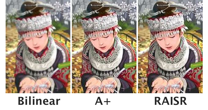
Super-resolution imaging is a class of techniques that enhance the resolution of an imaging system (Wikipedia). The entertainment series CSI has been ridiculed for relying on exaggerated and unrealistic applications of it:
As a result, there are now several applications where machines have learned to literallyfill in the blanks in imagery. Most notable seems the method developed by Google: Rapid and Accurate Image Super Resolution, or RAISR is short. In contrast to other approaches, RAISR does not rely on (adversarial) neural network(s) and is thus not as resource-demanding to train. Moreover, it’s performance is quite remarkable:
I guess you’re eager to test this super resolution out yourself?! letsenhance.io let’s you enhance the resolution of five images for free, after which it charges you $5 per twenty pictures processed. The website feeds the input image to a neural net and puts out an image of which the resolution has been increased four fold! I tested it with this random blurry picture I retrieved from Google/Pinterest.
Original 500×500
Enhanced 2000×2000
Do you see how much more detailed (though still blurry) the second image is? Nevertheless, upscaling four times seems about the limit as that is the default factor for both RAISR and Let’s Enhance. I am very curious to see how this super resolution is going to develop in the future, how it will be used to decrease memory or network demands, whether it will be integrated with video platforms like YouTube or Netflix, and which algorithm will ultimately take the crown!
Sorting is one of the central topic in most Computer Science degrees. In general, sorting refers to the process of rearranging data according to a defined pattern with the end goal of transforming the original unsorted sequence into a sorted sequence. It lies at the heart of successful businesses ventures — such as Google and Amazon — but is also present in many applications we use daily — such as Excel or Facebook.
Many different algorithms have been developed to sort data. Wikipedia lists as many as 45 and there are probably many more. Some work by exchanging data points in a sequence, others insert and/or merge parts of the sequence. More importantly, some algorithms are quite effective in terms of the time they take to sort data — taking only time to sort datapoints — whereas others are very slow — taking as much as . Moreover, some algorithms are stable — in the sense that they always take the same amount of time to process datapoints — whereas others may fluctuate in terms of processing time based on the original order of the data.
I really enjoyed this video by TED-Ed on how to best sort your book collection. It provides a very intuitive introduction into sorting strategies (i.e., algorithms). Moreover, Algorithms to Live By (Christian & Griffiths, 2016) provided the amazing suggestion to get friends and pizza in whenever you need to sort something, next to the great explanation of various algorithms and their computational demand.
The main reason for this blog is that I stumbled across some nice video’s and GIFs of sorting algorithms in action. These visualizations are not only wonderfully intriguing to look at, but also help so much in understanding how the sorting algorithms process the data under the hood. You might want to start with the 4-minute YouTube video below, demonstrating how nine different sorting algorithms (Selection Sort, Shell Sort, Insertion Sort, Merge Sort, Quick Sort, Heap Sort, Bubble Sort, Comb Sort, & Cocktail Sort) process a variety of datasets.
This interactive website toptal.com allows you to play around with the most well-known sorting algorithms, putting them to work on different datasets. For the grande finale, I found these GIFs and short video’s of several sorting algorithms on imgur. In the visualizations below, each row of the image represents an independent list being sorted. You can see that Bubble Sort is quite slow:
Cocktail Shaker Sort already seems somewhat faster, but still takes quite a while.
For some algorithms, the visualization clearly shows that the settings you pick matter. For instance, Heap Sort is much quicker if you choose to shift down instead of up.
In contrast, for Merge Sort it doesn’t matter whether you sort by breadth first or depth first.
The imgur overview includes many more visualized sorting algorithms but I don’t want to overload WordPress or your computer, so I’ll leave you with two types of Radix Sort, the rest you can look up yourself!


 You can read more details in the


 time to sort
  . Moreover, some algorithms are stable — in the sense that they always take the same amount of time to process