Robert Martin’s book Clean Code has been on my to-read list for months now. Browsing the web, I stumbled across this repository of where Ryan McDermott applied the book’s principles to JavaScript. Basically, he made a guide to producing readable, reusable, and refactorable software code in JavaScript.
Although Ryan’s good and bad code examples are written in JavaScript, the basic principles (i.e. “Uncle Bob”‘s Clean Code principles) are applicable to any programming language. At least, I recognize many of the best practices I’d teach data science students in R or Python.
Knowing these won’t immediately make you a better software developer, and working with them for many years doesn’t mean you won’t make mistakes. Every piece of code starts as a first draft, like wet clay getting shaped into its final form. Finally, we chisel away the imperfections when we review it with our peers. Don’t beat yourself up for first drafts that need improvement. Beat up the code instead!
YouTube recommended I’d watch this recorded presentation by Raymond Hettinger at PyBay2019 last October. Quite a long presentation for what I’d normally watch, but what an eye-openers it contains!
Raymond Hettinger is a Python core developer and in this video he presents 10 programming strategies in these 60 minutes, all using live examples. Some are quite obvious, but the presentation and examples make them very clear. Raymond presents some serious programming truths, and I think they’ll stick.
First, Raymond discusses chunking and aliasing. He brings up the theory that the human mind can only handle/remember 7 pieces of information at a time, give or take 2. Anything above proves to much cognitive load, and causes discomfort as well as errors. Hence, in a programming context, we need to make sure programmers can use all 7 to improve the code, rather than having to decypher what’s in front of them. In a programming context, we do so by modularizing and standardizing through functions, modules, and packages. Raymond uses the Python random module to hightlight the importance of chunking and modular code. This part was quite long, but still interesting.
For the next two strategies, Raymond quotes the Feinmann method of solving problems: “(1) write down a clear problem specification; (2) think very, very hard; (3) write down a solution”. Using the example of a tree walker, Raymond shows how the strategies of incremental development and solving simpler programs can help you build programs that solve complex problems. This part only lasts a couple of minutes but really underlines the immense value of these strategies.
Next, Raymond touches on the DRY principle: Don’t Repeat Yourself. But in a context I haven’t seen it in yet, object oriented programming [OOP], classes, and inherintance.
Raymond continues to build his arsenal of programming strategies in the next 10 minutes, where he argues that programmers should repeat tasks manually until patterns emerge, before they starting moving code into functions. Even though I might not fully agree with him here, he does have some fun examples of file conversion that speak in his case.
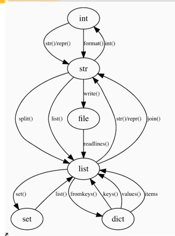
Lastly, Raymond uses the graph below to make the case that OOP is a graph traversal problem. According to Raymond, the Python ecosystem is so rich that there’s often no need to make new classes. You can simply look at the graph below. Look for the island you are currently on, check which island you need to get to, and just use the methods that are available, or write some new ones.
While there were several more strategies that Raymond wanted to discuss, he doesn’t make it to the end of his list of strategies as he spend to much time on the first, chunking bit. Super curious as to the rest? Contact Raymond on Twitter.
The R for Data Science (R4DS) book by Hadley Wickham is a definite must-read for every R programmer. Amongst others, the power of functional programming is explained in it very well in the chapter on Iteration. I wrote about functional programming before, but I recently re-read the R4DS book section after coming across some new valuable resources on particularly R’s purrr functions.
The purpose of this blog post is twofold. First, I wanted to share these new resources I came across, along with the other resources I already have collected over time on functional programming. Second, I wanted to demonstrate via code why functional programming is so powerful, and how it can speed up, clean, and improve your own workflow.
1. Resources
So first things first, “what are these new functional programming resources?”, you must be wondering. Well, here they are:
Thomas Mock was as inspired by the R4DS book as I was, and will run you through the details behind some of the examples in this tutorial.
Hadley Wickham himself gave a talk at a 2016 EdinbR meetup, explaing why and how to (1) use tidyr to make nested data frame, (2) use purrr for functional programming instead of for loops, and (3) visualise models by converting them to tidy data with broom:
Via YouTube.
Colin Fay dedicated several blogs to purrr. Some are very helpful as introduction — particularly this one — others demonstrate more expert applications of the power of purrr — such as this sequence of six blogs on web mining.
This GitHub repository by Dan Ovando does a fantastic job of explaining functional programming and demonstrating the functionality of purrr.
Cormac Nolan made a beautiful RPub Markdown where he displays how functional programming in combination with purrr‘s functions can result in very concise, fast, and supercharged code.
Last, but not least, part of Duke University 2017’s statistical programming course can be found here, related to functional programming with and without purrr.
2. Functional programming example
I wanted to run you through the basics behind functional programming, the apply family and their purrring successors. I try to do so by providing you some code which you can run in R yourself alongside this read. The content is very much inspired on the R4DS book chapter on iteration.
Let’s start with some data
# let's grab a subset of the mtcars dataset
mtc <- mtcars[ , 1:3] # store the first three columns in a new object
Say we would like to know the average (mean) value of the data in each of the columns of this new dataset. A starting programmer would usually write something like the below:
#### basic approach:

mean(mtc$mpg)
mean(mtc$cyl)
mean(mtc$disp)
However, this approach breaks therule of three! Bascially, we want to avoid copying and pasting anything more than twice.
A basic solution would be to use a for-loop to iterate through each column’s data one by one, and calculate and store the mean for each. Here, we first want to pre-allocate an output vector, in order to prevent that we grow (and copy into memory) a vector in each of the iterations of our for-loop. Details regarding why you do not want to grow a vector can be found here. A similar memory-issue you can create with for-loops is described here.
In the end, our for-loop approach to calculating column means could look something like this:
#### for loop approach:

output <- vector("double", ncol(mtc)) # pre-allocate an empty vector

# replace each value in the vector by the column mean using a for loop
for(i in seq_along(mtc)){
  output[i] <- mean(mtc[[i]])
}

# print the output
output
[1] 20.09062 6.18750 230.72188
This output is obviously correct, and the for-loop does the job, however, we are left with some unnecessary data created in our global environment, which not only takes up memory, but also creates clutter.
ls() # inspect global environment
[1] "i" "mtc" "output"
Let’s remove the clutter and move on.
rm(i, output) # remove clutter
Now, R is a functional programming language so this means that we can write our own function with for-loops in it! This way we prevent the unnecessary allocation of memory to overhead variables like i and output. For instance, take the example below, where we create a custom function to calculate the column means. Note that we still want to pre-allocate a vector to store our results.
#### functional programming approach:

col_mean <- function(df) {
  output <- vector("double", length(df))
  for (i in seq_along(df)) {
    output[i] <- mean(df[[i]])
  }
  output
}
Now, we can call this standardized piece of code by calling the function in different contexts:
This way we prevent that we have to write the same code multiple times, thus preventing errors and typos, and we are sure of a standardized output.
Moreover, this functional programming approach does not create unnecessary clutter in our global environment. The variables created in the for loop (i and output) only exist in the local environment of the function, and are removed once the function call finishes. Check for yourself, only our dataset and our user-defined function col_mean remain:
ls()
[1] "col_mean" "mtc"
For the specific purpose we are demonstrating here, a more flexible approach than our custom function already exists in base R: in the form of the apply family. It’s a set of functions with internal loops in order to “apply” a function over the elements of an object. Let’s look at some example applications for our specific problem where we want to calculate the mean values for all columns of our dataset.
#### apply approach:

# apply loops a function over the margin of a dataset
apply(mtc, MARGIN = 1, mean) # either by its rows (MARGIN = 1)
apply(mtc, MARGIN = 2, mean) # or over the columns (MARGIN = 2)

# in both cases apply returns the results in a vector
# sapply loops a function over the columns, returning the results in a vector
sapply(mtc, mean)
  mpg       cyl      disp
20.09062   6.18750 230.72188
# lapply loops a function over the columns, returning the results in a list
lapply(mtc, mean)
Sidenote: sapply and lapply both loop their input function over a dataframe’s columns by default as R dataframes are actually lists of equal-length vectors (see Advanced R [Wickham, 2014]).
# tapply loops a function over a vector
# grouping it by a second INDEX vector
# and returning the results in a vector
tapply(mtc$mpg, INDEX = mtc$cyl, mean)
   4        6        8
26.66364 19.74286 15.10000
These apply functions are a cleaner approach than the prior for-loops, as the output is more predictable (standard a vector or a list) and no unnecessary variables are allocated in our global environment.
Performing the same action to each element of an object and saving the results is so common in programming that our friends at RStudio decided to create the purrr package. It provides another family of functions to do these actions for you in a cleaner and more versatile approach building on functional programming.
install.packages("purrr")
library("purrr")
Like the apply family, there are multiple functions that each return a specific output:
# map_lgl returns a logical vector
# as numeric means aren't often logical, I had to call a different function
map_lgl(mtc, is.logical) # mtc's columns are numerical, hence FALSE
mpg   cyl  disp
FALSE FALSE FALSE
# map_int returns an integer vector
# as numeric means aren't often integers, I had to call a different function
map_int(mtc, is.integer) # returned FALSE, which is converted to integer (0)
mpg  cyl disp
  0    0    0
#map_dbl returns a double vector.
map_dbl(mtc, mean)
  mpg       cyl      disp
20.09062   6.18750 230.72188
# map_chr returns a character vector.
map_chr(mtc, mean)
     mpg          cyl         disp
"20.090625"   "6.187500" "230.721875"
All purrr functions are implemented in C. This makes them a little faster at the expense of readability. Moreover, the purrr functions can take in additional arguments. For instance, in the below example, the na.rm argument is passed to the mean function
map_dbl(rbind(mtc, c(NA, NA, NA)), mean) # returns NA due to the row of missing values
map_dbl(rbind(mtc, c(NA, NA, NA)), mean, na.rm = TRUE) # handles those NAs
mpg  cyl disp
 NA   NA   NA

     mpg       cyl      disp
20.09062   6.18750 230.72188
Once you get familiar with purrr, it becomes a very powerful tool. For instance, in the below example, we split our little dataset in groups for cyl and then run a linear model within each group, returning these models as a list (standard output of map). All with only three lines of code!
We can expand this as we go, for instance, by inputting this list of linear models into another map function where we run a model summary, and then extract the model coefficient using another subsequent map:
mtc %>% split(.$cyl) %>% map(~ lm(mpg ~ disp, data = .)) %>% map(summary) %>% # returns a list of linear model summaries map("coefficients")
$4
              Estimate Std. Error   t value     Pr(>|t|)
(Intercept) 40.8719553 3.58960540 11.386197 1.202715e-06
disp        -0.1351418 0.03317161 -4.074021 2.782827e-03
$6
                Estimate Std. Error   t value    Pr(>|t|)
(Intercept) 19.081987419 2.91399289 6.5483988 0.001243968
disp         0.003605119 0.01555711 0.2317344 0.825929685
$8
               Estimate  Std. Error   t value     Pr(>|t|)
(Intercept) 22.03279891 3.345241115  6.586311 2.588765e-05
disp        -0.01963409 0.009315926 -2.107584 5.677488e-02
The possibilities are endless, our code is fast and readable, our function calls provide predictable return values, and our environment stays clean!
PS. sorry for the terrible layout but WordPress really has been acting up lately… I really should move to some other blog hosting method. Any tips? Potentially Jekyll?
I recently came across this lovely article where Ali Spittel provides 7 tips for writing cleaner JavaScript code. Enthusiastic about her guidelines, I wanted to translate them to the R programming environment. However, since R is not an object-oriented programming language, not all tips were equally relevant in my opinion. Here’s what really stood out for me.
Suppose we want to create our own custom function to derive the average value of a vector v (please note that there is a base::mean function to do this much more efficiently). We could use the R code below to compute that the average of vector 1 through 10 is 5.5.
avg <- function(v){
    s = 0
    for(i in seq_along(v)) {
        s = s + v[i]
    }
    return(s / length(v))
}

avg(1:10) # 5.5
However, Ali rightfully argues that this code can be improved by making the variable and function names much more explicit. For instance, the refigured code below makes much more sense on a first look, while doing exactly the same.
averageVector <- function(vector){
    sum = 0
    for(i in seq_along(vector)){
        sum = sum + vector[i]
    }
    return(sum / length(vector))
}

averageVector(1:10) #5.5
Of course, you don’t want to make variable and function names unnecessary long (e.g., average would have been a great alternative function name, whereas computeAverageOfThisVector is probably too long). I like Ali’s principle:
Don’t minify your own code; use full variable names that the next developer can understand.
2. Write short functions that only do one thing
Ali argues “Functions are more understandable, readable, and maintainable if they do one thing only. If we have a bug when we write short functions, it is usually easier to find the source of that bug. Also, our code will be more reusable.” It thus helps to break up your code into custom functions that all do one thing and do that thing good!
For instance, our earlier function averageVector actually did two things. It first summated the vector, and then took the average. We can split this into two seperate functions in order to standardize our operations.
sumVector <- function(vector){
    sum = 0
    for(i in seq_along(vector)){
        sum = sum + vector[i]
    }
    return(sum)
}

averageVector <- function(vector){
    sum = sumVector(vector)
    average = sum / length(vector)
    return(average)
}

sumVector(1:10) # 55
averageVector(1:10) # 5.5
If you are writing a function that could be named with an “and” in it — it really should be two functions.
3. Documentation
Personally, I am terrible in commenting and documenting my work. I am always too much in a hurry, I tell myself. However, no more excuses! Anybody should make sure to write good documentation for their code so that future developers, including future you, understand what your code is doing and why!
Ali uses the following great example, of a piece of code with magic numbers in it.
Now, you might immediately recognize the number Pi in this return statement, but others may not. And maybe you will need the value Pi somewhere else in your script as well, but you accidentally use three decimals the next time. Best to standardize and comment!
PI <- 3.14 # PI rounded to two decimal places

areaOfCircle <- function(radius) {
  # Implements the mathematical equation for the area of a circle:
  # Pi times the radius of the circle squared.
  return(PI * radius ** 2)
}
The above is much clearer. And by making PI a variable, you make sure that you use the same value in other places in your script! Unfortunately, R doesn’t handle constants (unchangeable variables), but I try to denote my constants by using ALL CAPITAL variable names such as PI, MAX_GROUP_SIZE, or COLOR_EXPERIMENTAL_GROUP.
Do note that R has a built in variable pi for purposes such as the above.
I love Ali’s general rule that:
Your comments should describe the “why” of your code.
However, more elaborate R programming commenting guidelines are given in the Google R coding guide, stating that:
Functions should contain a comments section immediately below the function definition line. These comments should consist of a one-sentence description of the function; a list of the function’s arguments, denoted by Args:, with a description of each (including the data type); and a description of the return value, denoted by Returns:. The comments should be descriptive enough that a caller can use the function without reading any of the function’s code.
Either way, prevent that your comments only denote “what” your code does:
# EXAMPLE OF BAD COMMENTING ####

PI <- 3.14 # PI

areaOfCircle <- function(radius) {
    # custom function for area of circle
    return(PI * radius ** 2) # radius squared times PI
}
5. Be Consistent
I do not have as strong a sentiment about consistency as Ali does in her article, but I do agree that it’s nice if code is at least somewhat in line with the common style guides. For R, I like to refer to my R resources list which includes several common style guides, such as Google’s or Hadley Wickham’s Advanced R style guide.
For fresh R programmers, vectorization can sound awfully complicated. Consider two math problems, one vectorized, and one not:
Two ways of doing the same computations in R
Why on earth should R spend more time calculating one over the other? In both cases there are the same three addition operations to perform, so why the difference? This is what we will try to illustrate in this post, which is inspired on work by Naom Ross and the University of Auckland.
R behind the scenes:
R is a high-level, interpreted computer language. This means that R takes care of a lot of basic computer tasks for you. For instance, when you type i <- 5.0 you don’t have to tell R:
That 5.0 is a floating-point number
That i should store numeric-type data
To find a place in memory for to put 5
To register i as a pointer to that place in memory
You also don’t have to convert i <- 5.0 to binary code. That’s done automatically when you hit Enter. Although you are probably not aware of this, many R functions are just wrapping your input and passing it to functions of other, compiled computer languages, like C, C++, or FORTRAN, in the back end.
Now here’s the crux: If you need to run a function over a set of values, you can either pass in a vector of these values through the R function to the compiled code (math example 1), or you could call the R function repeatedly for each value separately (math example 2). If you do the latter, R has to do stuff (figuring out the above bullet points and translating the code) each time, repeatedly. However, if you call the function with a vector instead, this figuring out part only happens once. For instance, R vectors are constricted to a single data type (e.g., numeric, character) and when you use a vector instead of seperate values, R only needs to determine the input data type once, which saves time. In short, there’s no advantage to NOT organizing your data as vector.
For-loops and functional programming (*ply)
One example of how new R programmers frequently waste computing time is via memory allocation. Take the below for loop, for instance:
iterations = 10000000

 system.time({
   j = c()
   for(i in 1:iterations){
     j[i] <- i
   }
 })
##    user  system elapsed
##    3.71    0.23    3.94
Here, vector j starts out with length 1, but for each iteration in the for loop, R has to re-size the vector and re-allocate memory. Recursively, R has to find the vector in its memory, create a new vector that will fit more data, copy the old data over, insert the new data, and erase the old vector. This process gets very slow as vectors get big. Nevertheless, it is often how programmers store the results of their iterative processes. Tremendous computing power can be saved by pre-allocating vectors to fit all the values beforehand, so that R does not have to do unnecessary actions:
system.time({
   j = rep(NA, iterations)
   for(i in 1:iterations){
     j[i] <- i
   }
 })
##    user  system elapsed
##    0.88    0.01    0.89
More advanced R users tend to further optimize via functionals. This family of functions takes in vectors (or matrices, or lists) of values and applies other functions to each. Examples are apply or plyr::*ply functions, which speed up R code mainly because the for loops they have inside them automatically do things like pre-allocating vector size. Functionals additionally prevent side effects: unwanted changes to your working environment, such as the remaining i after for(i in 1:10). Although this does not necessarily improve computing time, it is regarded best practice due to preventing consequent coding errors.
Conclusions
There are cases when you should use for loops. For example, the performance penalty for using a for loop instead a vector will be small if the number of iterations is relatively small, and the functions called inside your for loop are slow. Here, looping and overhead from function calls make up a small fraction of your computational time and for loops may be more intuitive or easier to read for you. Additionally, there are cases where for loops make more sense than vectorized functions: (1) when the functions you seek to apply don’t take vector arguments and (2) when each iteration is dependent on the results of previous iterations.
Another general rule: fast R code is short. If you can express what you want to do in R in a line or two, with just a few function calls that are actually calling compiled code, it’ll be more efficient than if you write long program, with the added overhead of many function calls.
Finally, there is a saying that “premature optimization is the root of all evil”. What this means is that you should not re-write your R code unless the computing time you are going to save is worth the time invested. Nevertheless, if you understand how vectorization and functional programming work, you will be able to write more faster, safer, and more transparent (short & simple) programs.