Hugo Toscano wrote a great blog providing an overview of all the helpful functionalities of the R forcats package. The package includes functions that help handling categorical data, by setting a random or fixed order, and by recategorizing or anonymizing. These functions are specifically helpful when visualizing data with R’s ggplot2.
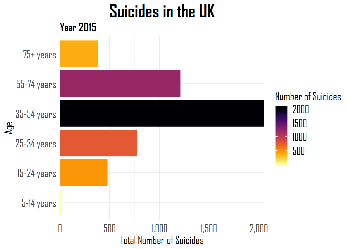
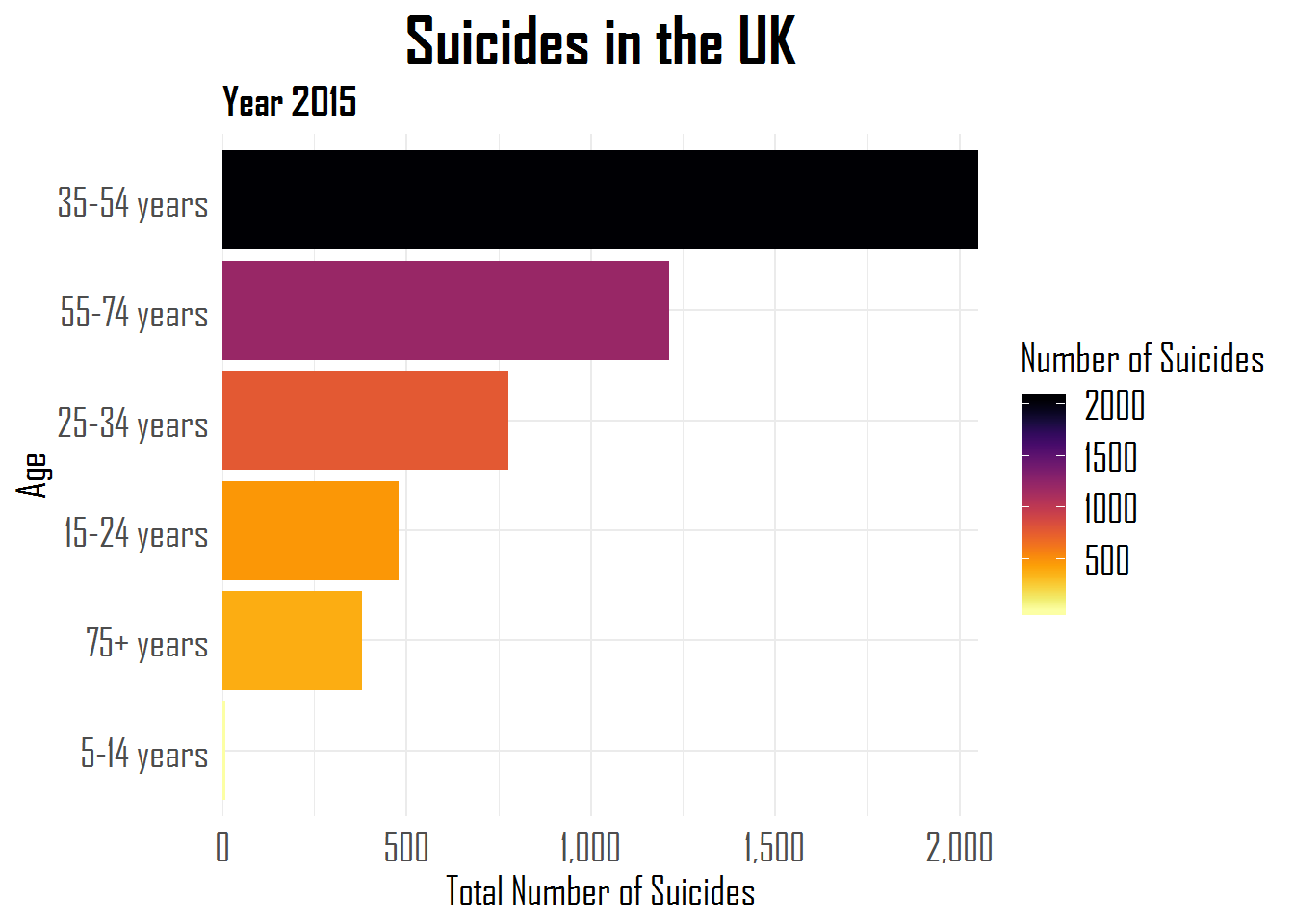
A comprehensive overview is provided in the form of the RStudio forcats cheat sheet, but, on his blog, Hugo demonstrates some of its functionalities using a dataset on suicides and people’s ages:
Other functions can be used to automatically surpress infrequent categories, to reverse the order of categories, to shuffle or shift categories, to quickly relabel or anonimize categories, and many more…
Fortunately, so much of the conference is shared on Twitter and media outlets that I still felt included. Here are some things that I liked and learned from, despite the Austin-Tilburg distance.
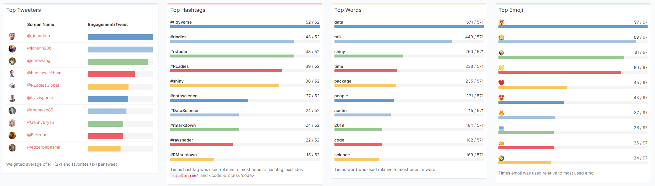
Garrick Aden-Buie made a fabulous Shiny app that allows you to review all #rstudioconf tweets during and since the conference. It even includes some random statistics about the tweets, and a page with all the shared media.
Data scientists can fail by: ❌not saying no enough ❌not providing anything more than a cursory analysis ❌assuming PM knows enough to ask question in the right way and not collaborating with them ❌caring more about using fancy method than solving business problems#rstudioconf
Did you know that RStudio also posts all the webinars they host? There really are some hidden pearls among them. For instance, this presentation by Nathan Stephens on rendering rmarkdown to powerpoint will save me tons of work, and those new to broom will also be astonished by this webinar by Alex Hayes.
The R for Data Science (R4DS) book by Hadley Wickham is a definite must-read for every R programmer. Amongst others, the power of functional programming is explained in it very well in the chapter on Iteration. I wrote about functional programming before, but I recently re-read the R4DS book section after coming across some new valuable resources on particularly R’s purrr functions.
The purpose of this blog post is twofold. First, I wanted to share these new resources I came across, along with the other resources I already have collected over time on functional programming. Second, I wanted to demonstrate via code why functional programming is so powerful, and how it can speed up, clean, and improve your own workflow.
1. Resources
So first things first, “what are these new functional programming resources?”, you must be wondering. Well, here they are:
Thomas Mock was as inspired by the R4DS book as I was, and will run you through the details behind some of the examples in this tutorial.
Hadley Wickham himself gave a talk at a 2016 EdinbR meetup, explaing why and how to (1) use tidyr to make nested data frame, (2) use purrr for functional programming instead of for loops, and (3) visualise models by converting them to tidy data with broom:
Via YouTube.
Colin Fay dedicated several blogs to purrr. Some are very helpful as introduction — particularly this one — others demonstrate more expert applications of the power of purrr — such as this sequence of six blogs on web mining.
This GitHub repository by Dan Ovando does a fantastic job of explaining functional programming and demonstrating the functionality of purrr.
Cormac Nolan made a beautiful RPub Markdown where he displays how functional programming in combination with purrr‘s functions can result in very concise, fast, and supercharged code.
Last, but not least, part of Duke University 2017’s statistical programming course can be found here, related to functional programming with and without purrr.
2. Functional programming example
I wanted to run you through the basics behind functional programming, the apply family and their purrring successors. I try to do so by providing you some code which you can run in R yourself alongside this read. The content is very much inspired on the R4DS book chapter on iteration.
Let’s start with some data
# let's grab a subset of the mtcars dataset
mtc <- mtcars[ , 1:3] # store the first three columns in a new object
Say we would like to know the average (mean) value of the data in each of the columns of this new dataset. A starting programmer would usually write something like the below:
#### basic approach:

mean(mtc$mpg)
mean(mtc$cyl)
mean(mtc$disp)
However, this approach breaks therule of three! Bascially, we want to avoid copying and pasting anything more than twice.
A basic solution would be to use a for-loop to iterate through each column’s data one by one, and calculate and store the mean for each. Here, we first want to pre-allocate an output vector, in order to prevent that we grow (and copy into memory) a vector in each of the iterations of our for-loop. Details regarding why you do not want to grow a vector can be found here. A similar memory-issue you can create with for-loops is described here.
In the end, our for-loop approach to calculating column means could look something like this:
#### for loop approach:

output <- vector("double", ncol(mtc)) # pre-allocate an empty vector

# replace each value in the vector by the column mean using a for loop
for(i in seq_along(mtc)){
  output[i] <- mean(mtc[[i]])
}

# print the output
output
[1] 20.09062 6.18750 230.72188
This output is obviously correct, and the for-loop does the job, however, we are left with some unnecessary data created in our global environment, which not only takes up memory, but also creates clutter.
ls() # inspect global environment
[1] "i" "mtc" "output"
Let’s remove the clutter and move on.
rm(i, output) # remove clutter
Now, R is a functional programming language so this means that we can write our own function with for-loops in it! This way we prevent the unnecessary allocation of memory to overhead variables like i and output. For instance, take the example below, where we create a custom function to calculate the column means. Note that we still want to pre-allocate a vector to store our results.
#### functional programming approach:

col_mean <- function(df) {
  output <- vector("double", length(df))
  for (i in seq_along(df)) {
    output[i] <- mean(df[[i]])
  }
  output
}
Now, we can call this standardized piece of code by calling the function in different contexts:
This way we prevent that we have to write the same code multiple times, thus preventing errors and typos, and we are sure of a standardized output.
Moreover, this functional programming approach does not create unnecessary clutter in our global environment. The variables created in the for loop (i and output) only exist in the local environment of the function, and are removed once the function call finishes. Check for yourself, only our dataset and our user-defined function col_mean remain:
ls()
[1] "col_mean" "mtc"
For the specific purpose we are demonstrating here, a more flexible approach than our custom function already exists in base R: in the form of the apply family. It’s a set of functions with internal loops in order to “apply” a function over the elements of an object. Let’s look at some example applications for our specific problem where we want to calculate the mean values for all columns of our dataset.
#### apply approach:

# apply loops a function over the margin of a dataset
apply(mtc, MARGIN = 1, mean) # either by its rows (MARGIN = 1)
apply(mtc, MARGIN = 2, mean) # or over the columns (MARGIN = 2)

# in both cases apply returns the results in a vector
# sapply loops a function over the columns, returning the results in a vector
sapply(mtc, mean)
  mpg       cyl      disp
20.09062   6.18750 230.72188
# lapply loops a function over the columns, returning the results in a list
lapply(mtc, mean)
Sidenote: sapply and lapply both loop their input function over a dataframe’s columns by default as R dataframes are actually lists of equal-length vectors (see Advanced R [Wickham, 2014]).
# tapply loops a function over a vector
# grouping it by a second INDEX vector
# and returning the results in a vector
tapply(mtc$mpg, INDEX = mtc$cyl, mean)
   4        6        8
26.66364 19.74286 15.10000
These apply functions are a cleaner approach than the prior for-loops, as the output is more predictable (standard a vector or a list) and no unnecessary variables are allocated in our global environment.
Performing the same action to each element of an object and saving the results is so common in programming that our friends at RStudio decided to create the purrr package. It provides another family of functions to do these actions for you in a cleaner and more versatile approach building on functional programming.
install.packages("purrr")
library("purrr")
Like the apply family, there are multiple functions that each return a specific output:
# map_lgl returns a logical vector
# as numeric means aren't often logical, I had to call a different function
map_lgl(mtc, is.logical) # mtc's columns are numerical, hence FALSE
mpg   cyl  disp
FALSE FALSE FALSE
# map_int returns an integer vector
# as numeric means aren't often integers, I had to call a different function
map_int(mtc, is.integer) # returned FALSE, which is converted to integer (0)
mpg  cyl disp
  0    0    0
#map_dbl returns a double vector.
map_dbl(mtc, mean)
  mpg       cyl      disp
20.09062   6.18750 230.72188
# map_chr returns a character vector.
map_chr(mtc, mean)
     mpg          cyl         disp
"20.090625"   "6.187500" "230.721875"
All purrr functions are implemented in C. This makes them a little faster at the expense of readability. Moreover, the purrr functions can take in additional arguments. For instance, in the below example, the na.rm argument is passed to the mean function
map_dbl(rbind(mtc, c(NA, NA, NA)), mean) # returns NA due to the row of missing values
map_dbl(rbind(mtc, c(NA, NA, NA)), mean, na.rm = TRUE) # handles those NAs
mpg  cyl disp
 NA   NA   NA

     mpg       cyl      disp
20.09062   6.18750 230.72188
Once you get familiar with purrr, it becomes a very powerful tool. For instance, in the below example, we split our little dataset in groups for cyl and then run a linear model within each group, returning these models as a list (standard output of map). All with only three lines of code!
We can expand this as we go, for instance, by inputting this list of linear models into another map function where we run a model summary, and then extract the model coefficient using another subsequent map:
mtc %>% split(.$cyl) %>% map(~ lm(mpg ~ disp, data = .)) %>% map(summary) %>% # returns a list of linear model summaries map("coefficients")
$4
              Estimate Std. Error   t value     Pr(>|t|)
(Intercept) 40.8719553 3.58960540 11.386197 1.202715e-06
disp        -0.1351418 0.03317161 -4.074021 2.782827e-03
$6
                Estimate Std. Error   t value    Pr(>|t|)
(Intercept) 19.081987419 2.91399289 6.5483988 0.001243968
disp         0.003605119 0.01555711 0.2317344 0.825929685
$8
               Estimate  Std. Error   t value     Pr(>|t|)
(Intercept) 22.03279891 3.345241115  6.586311 2.588765e-05
disp        -0.01963409 0.009315926 -2.107584 5.677488e-02
The possibilities are endless, our code is fast and readable, our function calls provide predictable return values, and our environment stays clean!
PS. sorry for the terrible layout but WordPress really has been acting up lately… I really should move to some other blog hosting method. Any tips? Potentially Jekyll?
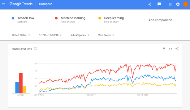
Tensorflow is a open-source machine learning (ML) framework. It’s primarily used to build neural networks, and thus very often used to conduct so-called deep learning through multi-layered neural nets.
Although there are other ML frameworks — such as Caffe or Torch — Tensorflow is particularly famous because it was developed by researchers of Google’s Brain Lab. There are widespread debates on which framework is best, nonetheless, Tensorflow does a pretty good job on marketing itself.
Google search engine searches on Tensorflow in comparison to searches on Machine learing and Deep learning
rstudio::conf is theyearly conference when it comes to R programming and RStudio. In 2017, nearly 500 people attended and, last week, 1100 people went to the 2018 edition. Regretfully, I was on holiday in Cardiff and missed out on meeting all my #rstats hero’s. Just browsing through the #rstudioconf Twitter-feed, I already learned so many new things that I decided to dedicate a page to it!
Fortunately, you can watch the live streams taped during the conference:
One of the workshops deserves an honorable mention. Jenny Bryan presented on What they forgot to teach you about R, providing some excellent advice on reproducible workflows. It elaborates on her earlier blog on project-oriented workflows, which you should read if you haven’t yet. Some best pRactices Jenny suggests:
Restart R often. This ensures your code is still working as intended. Use Shift-CMD-F10 to do so quickly in RStudio.
Use stable instead of absolute paths. This allows you to (1) better manage your imports/exports and folders, and (2) allows you to move/share your folders without the code breaking. For instance, here::here("data","raw-data.csv") loads the raw-data.csv-file from the data folder in your project directory. If you are not using the here package yet, you are honestly missing out! Alternatively you can use fs::path_home(). normalizePath() will make paths work on both windows and mac. You can usebasename instead of strsplit to get name of file from a path.
To upload an existing git directory to GitHub easily, you can usethis::use_github().
If you include the below YAML header in your .R file, you can easily generate .md files for you github repo.
#' ---
#' output: github_document
#' ---
Moreover, Jenny proposed these useful default settings for knitr:
Another of Jenny Bryan‘s talks was named Data Rectangling and although you might not get much out of her slides without her presenting them, you should definitely try the associated repurrrsivetutorial if you haven’t done so yet. It’s a poweR up for any useR!
I can’t remember who shared it, but a very cool trick is to name the viewing tab of any dataframe you pipe into View() using df %>% View("enter_view_tab_name").
These probably only present a minimal portion of the thousands of tips and tricks you could have learned by simply attending rstudio::conf. I will definitely try to attend next year’s edition. Nevertheless, I hope the above has been useful. If I missed out on any tips, presentations, tweets, or other materials, please reply below, tweet me or pop me a message!
This is reposted from DavisVaughan.com with minor modifications.
Introduction
A while back, I saw a conversation on twitter about how Hadley uses the word “pleased” very often when introducing a new blog post (I couldn’t seem to find this tweet anymore. Can anyone help?). Out of curiosity, and to flex my R web scraping muscles a bit, I’ve decided to analyze the 240+ blog posts that RStudio has put out since 2011. This post will do a few things:
Scrape the RStudio blog archive page to construct URL links to each blog post
Scrape the blog post text and metadata from each post
Use a bit of tidytext for some exploratory analysis
Perform a statistical test to compare Hadley’s use of “pleased” to the other blog post authors
To be able to extract the text from each blog post, we first need to have a link to that blog post. Luckily, RStudio keeps an up to date archive page that we can scrape. Using xml2, we can get the HTML off that page.
Now we use a bit of rvest magic combined with the HTML inspector in Chrome to figure out which elements contain the info we need (I also highly recommend SelectorGadget for this kind of work). Looking at the image below, you can see that all of the links are contained within the main tag as a tags (links).
The code below extracts all of the links, and then adds the prefix containing the base URL of the site.
links <- archive_html %>%
# Only the "main" body of the archive
html_nodes("main") %>%
# Grab any node that is a link
html_nodes("a") %>%
# Extract the hyperlink reference from those link tags# The hyperlink is an attribute as opposed to a node
html_attr("href") %>%
# Prefix them all with the base URL
paste0("http://blog.rstudio.com", .)
head(links)
Now that we have every link, we’re ready to extract the HTML from each individual blog post. To make things more manageable, we start by creating a tibble, and then using the mutate + map combination to created a column of XML Nodesets (we will use this combination a lot). Each nodeset contains the HTML for that blog post (exactly like the HTML for the archive page).
blog_data <- tibble(links)

blog_data <- blog_data %>%
  mutate(main = map(
                    # Iterate through every link
                    .x = links,

                    # For each link, read the HTML for that page, and return the main section
                    .f = ~read_html(.) %>%
                            html_nodes("main")
                    )
         )

select(blog_data, main)
Before extracting the blog post itself, lets grab the meta information about each post, specifically:
Author
Title
Date
Category
Tags
In the exploratory analysis, we will use author and title, but the other information might be useful for future analysis.
Looking at the first blog post, the Author, Date, and Title are all HTML class names that we can feed into rvest to extract that information.
In the code below, an example of extracting the author information is shown. To select a HTML class (like “author”) as opposed to a tag (like “main”), we have to put a period in front of the class name. Once the html node we are interested in has been identified, we can extract the text for that node using html_text().
Finally, notice that if we switch ".author" with ".title" or ".date" then we can grab that information as well. This kind of thinking means that we should create a function for extracting these pieces of information!
extract_info <- function(html, class_name) {
  map_chr(
          # Given the list of main HTMLs
          .x = html,

          # Extract the text we are interested in for each one
          .f = ~html_nodes(.x, class_name) %>%
                  html_text())
}

# Extract the data
blog_data <- blog_data %>%
  mutate(
     author = extract_info(main, ".author"),
     title  = extract_info(main, ".title"),
     date   = extract_info(main, ".date")
    )

select(blog_data, author, date)
## # A tibble: 249 x 2## author date## <chr> <chr>## 1 Jonathan McPherson 2017-08-16## 2 Hadley Wickham 2017-08-15## 3 Gary Ritchie 2017-08-11## 4 Roger Oberg 2017-08-10## 5 Jeff Allen 2017-08-03## 6 Javier Luraschi 2017-07-31## 7 Hadley Wickham 2017-07-13## 8 Roger Oberg 2017-07-12## 9 Garrett Grolemund 2017-07-11## 10 Hadley Wickham 2017-06-27## # ... with 239 more rows
select(blog_data, title)
## # A tibble: 249 x 1## title## <chr>## 1 RStudio 1.1 Preview - Data Connections## 2 rstudio::conf(2018): Contributed talks, e-posters, and diversity scholarshi## 3 RStudio v1.1 Preview: Terminal## 4 Building tidy tools workshop## 5 RStudio Connect v1.5.4 - Now Supporting Plumber!## 6 sparklyr 0.6## 7 haven 1.1.0## 8 Registration open for rstudio::conf 2018!## 9 Introducing learnr## 10 dbplyr 1.1.0## # ... with 239 more rows
Categories and tags
The other bits of meta data that might be interesting are the categories and tags that the post falls under. This is a little bit more involved, because both the categories and tags fall under the same class, ".terms". To separate them, we need to look into the href to see if the information is either a tag or a category (href = “/categories/” VS href = “/tags/”).
The function below extracts either the categories or the tags, depending on the argument, by:
Extracting the ".terms" class, and then all of the links inside of it (a tags).
Checking each link to see if the hyperlink reference contains “categories” or “tags” depending on the one that we are interested in. If it does, it returns the text corresponding to that link, otherwise it returns NAs which are then removed.
The final step results in two list columns containing character vectors of varying lengths corresponding to the categories and tags of each post.
extract_tag_or_cat <- function(html, info_name) {

  # Extract the links under the terms class
  cats_and_tags <- map(.x = html,
                       .f = ~html_nodes(.x, ".terms") %>%
                              html_nodes("a"))

  # For each link, if the href contains the word categories/tags
  # return the text corresponding to that link
  map(cats_and_tags,
    ~if_else(condition = grepl(info_name, html_attr(.x, "href")),
             true      = html_text(.x),
             false     = NA_character_) %>%
      .[!is.na(.)])
}

# Apply our new extraction function
blog_data <- blog_data %>%
  mutate(
    categories = extract_tag_or_cat(main, "categories"),
    tags       = extract_tag_or_cat(main, "tags")
  )

select(blog_data, categories, tags)
Finally, to extract the blog post itself, we can notice that each piece of text in the post is inside of a paragraph tag (p). Being careful to avoid the ".terms" class that contained the categories and tags, which also happens to be in a paragraph tag, we can extract the full blog posts. To ignore the ".terms" class, use the :not() selector.
blog_data <- blog_data %>%
  mutate(
    text = map_chr(main, ~html_nodes(.x, "p:not(.terms)") %>%
                 html_text() %>%
                 # The text is returned as a character vector.
                 # Collapse them all into 1 string.
                 paste0(collapse = " "))
  )

select(blog_data, text)
## # A tibble: 249 x 1## text## <chr>## 1 Today, we’re continuing our blog series on new features in RStudio 1.1. If ## 2 rstudio::conf, the conference on all things R and RStudio, will take place ## 3 Today we’re excited to announce availability of our first Preview Release f## 4 Have you embraced the tidyverse? Do you now want to expand it to meet your ## 5 We’re thrilled to announce support for hosting Plumber APIs in RStudio Conn## 6 We’re excited to announce a new release of the sparklyr package, available ## 7 "I’m pleased to announce the release of haven 1.1.0. Haven is designed to f## 8 RStudio is very excited to announce that rstudio::conf 2018 is open for reg## 9 We’re pleased to introduce the learnr package, now available on CRAN. The l## 10 "I’m pleased to announce the release of the dbplyr package, which now conta## # ... with 239 more rows
Who writes the most posts?
Now that we have all of this data, what can we do with it? To start with, who writes the most posts?
blog_data %>%
  group_by(author) %>%
  summarise(count = n()) %>%
  mutate(author = reorder(author, count)) %>%

  # Create a bar graph of author counts
  ggplot(mapping = aes(x = author, y = count)) +
  geom_col() +
  coord_flip() +
  labs(title    = "Who writes the most RStudio blog posts?",
       subtitle = "By a huge margin, Hadley!") +
  # Shoutout to Bob Rudis for the always fantastic themes
  hrbrthemes::theme_ipsum(grid = "Y")
Tidytext
I’ve never used tidytext before today, but to get our feet wet, let’s create a tokenized tidy version of our data. By using unnest_tokens() the data will be reshaped to a long format holding 1 word per row, for each blog post. This tidy format lends itself to all manner of analysis, and a number of them are outlined in Julia Silge and David Robinson’s Text Mining with R.
## # A tibble: 84,542 x 2## title word## <chr> <chr>## 1 RStudio 1.1 Preview - Data Connections today## 2 RStudio 1.1 Preview - Data Connections we’re## 3 RStudio 1.1 Preview - Data Connections continuing## 4 RStudio 1.1 Preview - Data Connections our## 5 RStudio 1.1 Preview - Data Connections blog## 6 RStudio 1.1 Preview - Data Connections series## 7 RStudio 1.1 Preview - Data Connections on## 8 RStudio 1.1 Preview - Data Connections new## 9 RStudio 1.1 Preview - Data Connections features## 10 RStudio 1.1 Preview - Data Connections in## # ... with 84,532 more rows
Remove stop words
A number of words like “a” or “the” are included in the blog that don’t really add value to a text analysis. These stop words can be removed using an anti_join() with the stop_words dataset that comes with tidytext. After removing stop words, the number of rows was cut in half!
As mentioned at the beginning of the post, Hadley apparently uses the word “pleased” in his blog posts an above average number of times. Can we verify this statistically?
Our null hypothesis is that the proportion of blog posts that use the word “pleased” written by Hadley is less than or equal to the proportion of those written by the rest of the RStudio team.
More simply, our null is that Hadley uses “pleased” less than or the same as the rest of the team.
Let’s check visually to compare the two groups of posts.
pleased <- tokenized_blog %>%
# Group by blog post
group_by(title) %>%
# If the blog post contains "pleased" put yes, otherwise no# Add a column checking if the author was Hadley
mutate(
contains_pleased = case_when(
"pleased" %in% word ~ "Yes",
TRUE ~ "No"),
is_hadley = case_when(
author == "Hadley Wickham" ~ "Hadley",
TRUE ~ "Not Hadley")
) %>%
# Remove all duplicates now
distinct(title, contains_pleased, is_hadley)
pleased %>%
ggplot(aes(x = contains_pleased)) +
geom_bar() +
facet_wrap(~is_hadley, scales = "free_y") +
labs(title = "Does this blog post contain 'pleased'?",
subtitle = "Nearly half of Hadley's do!",
x = "Contains 'pleased'",
y = "Count") +
hrbrthemes::theme_ipsum(grid = "Y")
Is there a statistical difference here?
To check if there is a statistical difference, we will use a test for difference in proportions contained in the R function, prop.test(). First, we need a continency table of the counts. Given the current form of our dataset, this isn’t too hard with the table() function from base R.
contingency_table <- pleased %>%
  ungroup() %>%
  select(is_hadley, contains_pleased) %>%
  # Order the factor so Yes is before No for easy interpretation
  mutate(contains_pleased = factor(contains_pleased, levels = c("Yes", "No"))) %>%
  table()

contingency_table
From our null hypothesis, we want to perform a one sided test. The alternative to our null is that Hadley uses “pleased” more than the rest of the RStudio team. For this reason, we specify alternative = "greater".
10.56% of the rest of the RStudio team’s posts contain “pleased”
With a p-value of 2.04e-11, we reject the null that Hadley uses “pleased” less than or the same as the rest of the team. The evidence supports the idea that he has a much higher preference for it!
Hadley uses “pleased” quite a bit!
About the author
Davis Vaughan is a Master’s student studying Mathematical Finance at the University of North Carolina at Charlotte. He is the other half of Business Science. We develop R packages for financial analysis. Additionally, we have a network of data scientists at our disposal to bring together the best team to work on consulting projects. Check out our website to learn more! He is the coauthor of R packages tidyquant and timetk.