Tag: javascript

7 tips for writing cleaner JavaScript code, translated to 3.5 tips for R programming

7 tips for writing cleaner JavaScript code, translated to 3.5 tips for R programming

I recently came across this lovely article where Ali Spittel provides 7 tips for writing cleaner JavaScript code. Enthusiastic about her guidelines, I wanted to translate them to the R programming environment. However, since R is not an object-oriented programming language, not all tips were equally relevant in my opinion. Here’s what really stood out for me.

Capture.PNG
Ali Spittel’s Javascript tips, via https://dev.to/aspittel/extreme-makeover-code-edition-k5k

1. Use clear variable and function names

Suppose we want to create our own custom function to derive the average value of a vector v (please note that there is a base::mean function to do this much more efficiently). We could use the R code below to compute that the average of vector 1 through 10 is 5.5.

avg <- function(v){
    s = 0
    for(i in seq_along(v)) {
        s = s + v[i]
    }
    return(s / length(v))
}

avg(1:10) # 5.5

However, Ali rightfully argues that this code can be improved by making the variable and function names much more explicit. For instance, the refigured code below makes much more sense on a first look, while doing exactly the same.

averageVector <- function(vector){
    sum = 0
    for(i in seq_along(vector)){
        sum = sum + vector[i]
    }
    return(sum / length(vector))
}

averageVector(1:10) #5.5

Of course, you don’t want to make variable and function names unnecessary long (e.g., average would have been a great alternative function name, whereas computeAverageOfThisVector is probably too long). I like Ali’s principle:

Don’t minify your own code; use full variable names that the next developer can understand.

2. Write short functions that only do one thing

Ali argues “Functions are more understandable, readable, and maintainable if they do one thing only. If we have a bug when we write short functions, it is usually easier to find the source of that bug. Also, our code will be more reusable.” It thus helps to break up your code into custom functions that all do one thing and do that thing good!

For instance, our earlier function averageVector actually did two things. It first summated the vector, and then took the average. We can split this into two seperate functions in order to standardize our operations.

sumVector <- function(vector){
    sum = 0
    for(i in seq_along(vector)){
        sum = sum + vector[i]
    }
    return(sum)
}

averageVector <- function(vector){
    sum = sumVector(vector)
    average = sum / length(vector)
    return(average)
}

sumVector(1:10) # 55
averageVector(1:10) # 5.5

If you are writing a function that could be named with an “and” in it — it really should be two functions.

3. Documentation

Personally, I am terrible in commenting and documenting my work. I am always too much in a hurry, I tell myself. However, no more excuses! Anybody should make sure to write good documentation for their code so that future developers, including future you, understand what your code is doing and why!

Ali uses the following great example, of a piece of code with magic numbers in it.

areaOfCircle <- function(radius) {
  return(3.14 * radius ** 2)
}

Now, you might immediately recognize the number Pi in this return statement, but others may not. And maybe you will need the value Pi somewhere else in your script as well, but you accidentally use three decimals the next time. Best to standardize and comment!

PI <- 3.14 # PI rounded to two decimal places

areaOfCircle <- function(radius) {
  # Implements the mathematical equation for the area of a circle:
  # Pi times the radius of the circle squared.
  return(PI * radius ** 2)
}

The above is much clearer. And by making PI a variable, you make sure that you use the same value in other places in your script! Unfortunately, R doesn’t handle constants (unchangeable variables), but I try to denote my constants by using ALL CAPITAL variable names such as PI, MAX_GROUP_SIZE, or COLOR_EXPERIMENTAL_GROUP.

Do note that R has a built in variable pi for purposes such as the above.

I love Ali’s general rule that:

Your comments should describe the “why” of your code.

However, more elaborate R programming commenting guidelines are given in the Google R coding guide, stating that:

Functions should contain a comments section immediately below the function definition line. These comments should consist of a one-sentence description of the function; a list of the function’s arguments, denoted by Args:, with a description of each (including the data type); and a description of the return value, denoted by Returns:. The comments should be descriptive enough that a caller can use the function without reading any of the function’s code.

Either way, prevent that your comments only denote “what” your code does:

# EXAMPLE OF BAD COMMENTING ####

PI <- 3.14 # PI

areaOfCircle <- function(radius) {
    # custom function for area of circle
    return(PI * radius ** 2) # radius squared times PI
}

5. Be Consistent

I do not have as strong a sentiment about consistency as Ali does in her article, but I do agree that it’s nice if code is at least somewhat in line with the common style guides. For R, I like to refer to my R resources list which includes several common style guides, such as Google’s or Hadley Wickham’s Advanced R style guide.


dygraphs

dygraphs

Today I learned about dygraphs, a fast, flexible open source JavaScript charting library. As everything in JavaScript, the charts produced by dygraphs integrate completely in the webbrowser and are thus very functional and interactive. See, for instance, the below where the graph highlights the y-axis value for both time series in the graph based on the x-axis value of my mouse location (January 24 2009). Very cool!

1.png

While I am no JS hero, the webpage includes a dypgrahs tutorial, as well as a playground environment.

Fortunately, I do know my way around R, and of course someone had already integrated dypgrahs in R in the form of the dygraphs R package. It works like a charm!

install.packages("dygraphs")
library("dygraphs")

dygraph(AirPassengers)

Also in R, your dygraphs are fully interactive, with my mouse hoevering over June 1951 in the below example.

2.PNG

And you can add all kinds of cool elements and modifications to the graphs, such as for instance a range selector:

dygraph(AirPassengers) %>% dyRangeSelector()

3.PNG

For the full range of visualization options dygraphs offers in R, please do have a look at the official RStudio page.

Bellwoods: A procedurally generated game in only 13 kilobytes

Bellwoods: A procedurally generated game in only 13 kilobytes

JS13K Games is a competition where developers are challenged to create an entire game using less than 13 kilobytes of memory. Creative developer Matt Deslaudiers participated and created Bellwoods: an art game for mobile and desktop that you can play in your browser.

The concept of the game is simple: fly your kite through endless fields of colour and sound, trying to discover new worlds. To remain under 13kb, all of the graphics and audio in Bellwoods are procedurally generated. The game was mostly programmed in JavaScript with minimal custom HTML/CSS. Matt’s motivation and the actual development you can read about in his original blog. The source code the game, Matt also shared on GitHub.

Mélissa Hernandez, a French UX and Interaction Designer, helped Matt design this beautiful game. Together, they even versed a haiku that not only evokes the mood of the game, but also provides some subtle gameplay instructions:

over the tall grass
following birds, chasing wind
in search of color

Play the game yourself, or have a quick look and feel with the video below.

Generating Pusheen with AI

Generating Pusheen with AI

Zack Nado wrote the best machine learning application I’ve seen so far: a neural network architecture that generates new Pusheen pictures.

Image result for pusheen
This is an orginal Pusheen picture.

In his blog, Zack describes his generative adversarial network (GAN) , a special type of machine learning architecture where two neural networks try to fool each other. Zack first gave the discriminator network some real Pusheen images, so it gets an idea of what Pusheen looks like. Next, the generator network gets a bunch of random numbers so it can generate completely new (fake) images. These generated images are then fed back into the discriminator, so it knows what generated images look like. Zack repeated this process several hundred thousand times, so he obtained a generator network that’s great at making new Pusheen images which the discriminator (nearly) can’t dinstinguish from the original, real ones. Below is the learning process of the generator network visualized:

ezgif.com-video-to-gif
Samples output by the generator network. It learns distinctive features of “real” Pusheen (e.g., tail, eyes, ears) over time [original]


In the end, the generated images are very much like the real Pusheen. Zack added an interactive module (using Tensorflow.js) to the blog so you can generate some Pusheens yourself. (it didn’t work for me though…) On a final note, Zack wrote the orginal blog both in plain English, for non-experts, and in jargon, for the more experienced data scientists. I highly recommend you read either one of those versions!

Some of the Pusheen’s generated by Zack’s GAN [original]

Job-Switching Behaviors in the USA

Job-Switching Behaviors in the USA

Nathan Yau – the guy behind the wonderful visualizations of FlowingData.com – has been looking into job market data more and more lately. For his latest project, he took data of the Current Population Survey (2011-2016) a survey run by the US Census Bureau and Bureau of Labor Statistics. This survey covers many topics, but Nathan specifically looked into people’s current occupation and what they were doing the year before.

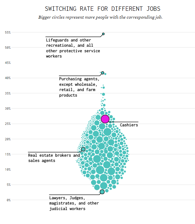
For his first visualization, Nathan examined the percentage of people switching jobs (a statistic he dubs the switching rate). Only occupations with over 100 survey responses are shown:

switchrate.png
Nathan concludes that jobs that come with higher salaries and require more training, education, and experience have lower switching rates. The interactive visualization can be found on FlowingData.com

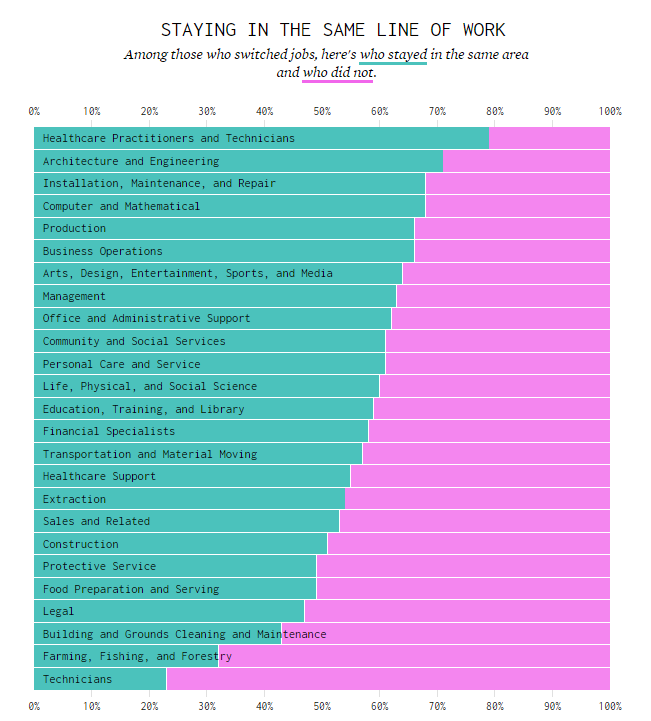
Next Nathan looked into job moves within job categories, as he hypothesizes that people who decide to switch jobs look for something similar.

switchcategories.png
Nathan concludes that job categories with lower entry boundaries are subjected to more leavers. Original on FlowingData.com

The above results in the main question of the blog: Given you have a certain job, what are the possible jobs to switch to? The following interactive bar charts gives the top 20 jobs people with a specific job switched to. In the original blog you can specify a job to examine or ask for a random suggestion. I searched for “analyst” in the picture below, and apparently HR professional would be a good next challenge.

switchchoices.png
The interactive visualization can be found on FlowingData.com

Nathan got the data here, prepared it in R, and used d3.js for the visualizations. I’d have loved to see this data in a network-kind of flowchart or a Markov-chain. For more of Nathan’s work, please visit his FlowingData website.

Visualizing Neural Networks in Processing

Visualizing Neural Networks in Processing

Coding Train is a Youtube channel by Daniel Shiffman that covers anything from the basics of programming languages like JavaScript (with p5.js) and Java (with Processing) to generative algorithms like physics simulation, computer vision, and data visualization. In particular, these latter topics, which Shiffman bundles under the label “the Nature of Code”, draw me to the channel.

In a recent series, Daniel draws from his free e-book to create his seven-video playlist where he elaborates on the inner workings of neural networks, visualizing the entire process as he programs the algorithm from scratch in Processing (Java). I recommend the two videos below consisting of the actual programming, especially for beginners who want to get an intuitive sense of how a neural network works.

PS. I tend to watch them on double speed.

Part 1:

Part 2: