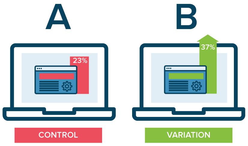
A/B testing is a method of comparing two versions of some thing against each other to determine which is better. A/B tests are often mentioned in e-commerce contexts, where the things we are comparing are web pages.
Business leaders and data scientists alike face a difficult trade-off when running A/B tests: How big should the A/B test be? Or in other words, After collecting how many data points, or running for how many days, should we make a decision whether A or B is the best way to go?
This is a tradeoff because the sample size of an A/B test determines its statistical power. This statistical power, in simple terms, determines the probability of a A/B test showing an effect if there is actually really an effect. In general, the more data you collect, the higher the odds of you finding the real effect and making the right decision.
By default, researchers often aim for 80% power, with a 5% significance cutoff. But is this general guideline really optimal for the tradeoff between costs and benefits in your specific business context? Chris thinks not.
Chris said wrote a great three-piece blog in which he explains how you can mathematically determine the optimal duration of A/B-testing in your own company setting:
Part I: General Overview. Starts with a mostly non-technical overview and ends with a section called “Three lessons for practitioners”.
Part II: Expected lift. A more technical section that quantifies the benefits of experimentation as a function of sample size.
Part III: Aggregate time-discounted lift. A more technical section that quantifies the costs of experimentation as a function of sample size. It then combines costs and benefits into a closed-form expression that can be optimized. Ends with an FAQ.
I recently visited a data science meetup where one of the speakers — Harm Bodewes — spoke about playing out the Monty Hall problem with his kids.
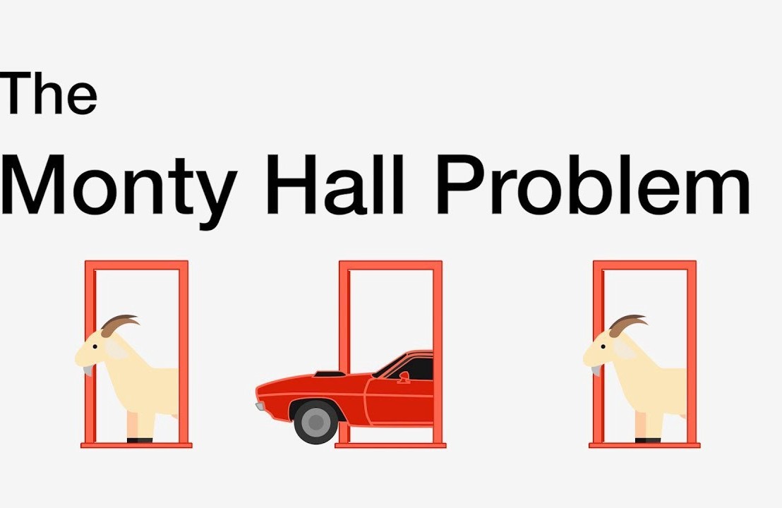
TheMonty Hall problemis probability puzzle. Based on the American television game show Let’s Make a Deal and its host, named Monty Hall:
You’re given the choice of three doors.
Behind one door sits a prize: a shiny sports car.
Behind the others doors, something shitty, like goats.
You pick a door — say, door 1.
Now, the host, who knows what’s behind the doors, opens one of the other doors — say, door 2 — which reveals a goat.
The host then asks you: Do you want to stay with door 1, or would you like to switch to door 3?
The probability puzzle here is:
Is switching doors the smart thing to do?
Back to my meetup.
Harm — the presenter — had ran the Monty Hall experiment with his kids.
Twenty-five times, he had hidden candy under one of three plastic cups. His kids could then pick a cup, he’d remove one of the non-candy cups they had not picked, and then he’d proposed them to make the switch.
The results he had tracked, and visualized in a simple Excel graph. And here he was presenting these results to us, his Meetup audience.
People (also statisticans) had been arguing whether it is best to stay or switch doors for years. Yet, here, this random guy ran a play-experiment and provided very visual proof removing any doubts you might have yourself.
You really need to switch doors!
At about the same time, I came across this Github repo by Saghir, who had made some vectorised simulations of the problem in R. I thought it was a fun excercise to simulate and visualize matters in two different data science programming languages — Python & R — and see what I’d run in to.
So I’ll cut to the chase.
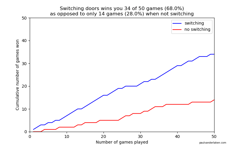
As we play more and more games against Monty Hall, it becomes very clear that you really, really, really need to switch doors in order to maximize the probability of winning a car.
Actually, the more games we play, the closer the probability of winning in our sample gets to the actual probability.
Even after 1000 games, the probabilities are still not at their actual values. But, ultimately…
If you stick to your door, you end up with the car in only 33% of the cases.
If you switch to the other door, you end up with the car 66% of the time!
Simulation Code
In both Python and R, I wrote two scripts. You can find the most recent version of the code on my Github. However, I pasted the versions of March 4th 2020 below.
The first script contains a function simulating a single game of Monty Hall. A second script runs this function an X amount of times, and visualizes the outcomes as we play more and more games.
Python
simulate_game.py
import random

def simulate_game(make_switch=False, n_doors=3, seed=None):
    '''
    Simulate a game of Monty Hall
    For detailed information: https://en.wikipedia.org/wiki/Monty_Hall_problem
    Basically, there are several closed doors and behind only one of them is a prize.
    The player can choose one door at the start.
    Next, the game master (Monty Hall) opens all the other doors, but one.
    Now, the player can stick to his/her initial choice or switch to the remaining closed door.
    If the prize is behind the player's final choice he/she wins.

    Keyword arguments:
    make_switch -- a boolean value whether the player switches after its initial choice and Monty Hall opening all other non-prize doors but one (default False)
    n_doors -- an integer value > 2, for the number of doors behind which one prize and (n-1) non-prizes (e.g., goats) are hidden (default 3)
    seed -- a seed to set (default None)
    '''

    # check the arguments
    if type(make_switch) is not bool:
        raise TypeError("`make_switch` must be boolean")
    if type(n_doors) is float:
        n_doors = int(n_doors)
        raise Warning("float value provided for `n_doors`: forced to integer value of", n_doors)
    if type(n_doors) is not int:
        raise TypeError("`n_doors` needs to be a positive integer > 2")
    if n_doors < 2:
        raise ValueError("`n_doors` needs to be a positive integer > 2")

    # if a seed was provided, set it
    if seed is not None:
        random.seed(seed)

    # sample one index for the door to hide the car behind
    prize_index = random.randint(0, n_doors - 1)

    # sample one index for the door initially chosen by the player
    choice_index = random.randint(0, n_doors - 1)

    # we can test for the current result
    current_result = prize_index == choice_index

    # now Monty Hall opens all doors the player did not choose, except for one door
    # next, he asks the player if he/she wants to make a switch
    if (make_switch):
        # if we do, we change to the one remaining door, which inverts our current choice
        # if we had already picked the prize door, the one remaining closed door has a nonprize
        # if we had not already picked the prize door, the one remaining closed door has the prize
        return not current_result
    else:
        # the player sticks with his/her original door,
        # which may or may not be the prize door
        return current_result
visualize_game_results.py
from simulate_game import simulate_game
from random import seed
from numpy import mean, cumsum
from matplotlib import pyplot as plt
import os

# set the seed here
# do not set the `seed` parameter in `simulate_game()`,
# as this will make the function retun `n_games` times the same results
seed(1)

# pick number of games you want to simulate
n_games = 1000

# simulate the games and store the boolean results
results_with_switching = [simulate_game(make_switch=True) for _ in range(n_games)]
results_without_switching = [simulate_game(make_switch=False) for _ in range(n_games)]

# make a equal-length list showing, for each element in the results, the game to which it belongs
games = [i + 1 for i in range(n_games)]

# generate a title based on the results of the simulations
title = f'Switching doors wins you {sum(results_with_switching)} of {n_games} games ({mean(results_with_switching) * 100:.1f}%)' + \
    '\n' + \
    f'as opposed to only {sum(results_without_switching)} games ({mean(results_without_switching) * 100:.1f}%) when not switching'

# set some basic plotting parameters
w = 8
h = 5

# make a line plot of the cumulative wins with and without switching
plt.figure(figsize=(w, h))
plt.plot(games, cumsum(results_with_switching), color='blue', label='switching')
plt.plot(games, cumsum(results_without_switching), color='red', label='no switching')
plt.axis([0, n_games, 0, n_games])
plt.title(title)
plt.legend()
plt.xlabel('Number of games played')
plt.ylabel('Cumulative number of games won')
plt.figtext(0.95, 0.03, 'paulvanderlaken.com', wrap=True, horizontalalignment='right', fontsize=6)

# you can uncomment this to see the results directly,
# but then python will not save the result to your directory
# plt.show()
# plt.close()

# create a directory to store the plots in
# if this directory does not yet exist
try:
    os.makedirs('output')
except OSError:
    None
plt.savefig('output/monty-hall_' + str(n_games) + '_python.png')
Visualizations (matplotlib)
R
simulate-game.R
Note that I wrote a second function, simulate_n_games, which just runs simulate_game an N number of times.
#' Simulate a game of Monty Hall
#' For detailed information: https://en.wikipedia.org/wiki/Monty_Hall_problem
#' Basically, there are several closed doors and behind only one of them is a prize.
#' The player can choose one door at the start.
#' Next, the game master (Monty Hall) opens all the other doors, but one.
#' Now, the player can stick to his/her initial choice or switch to the remaining closed door.
#' If the prize is behind the player's final choice he/she wins.
#'
#' @param make_switch A boolean value whether the player switches after its initial choice and Monty Hall opening all other non-prize doors but one. Defaults to `FALSE`
#' @param n_doors An integer value > 2, for the number of doors behind which one prize and (n-1) non-prizes (e.g., goats) are hidden. Defaults to `3L`
#' @param seed A seed to set. Defaults to `NULL`
#'
#' @return A boolean value indicating whether the player won the prize
#'
#' @examples
#' simulate_game()
#' simulate_game(make_switch = TRUE)
#' simulate_game(make_switch = TRUE, n_doors = 5L, seed = 1)
simulate_game = function(make_switch = FALSE, n_doors = 3L, seed = NULL) {

  # check the arguments
  if (!is.logical(make_switch) | is.na(make_switch)) stop("`make_switch` needs to be TRUE or FALSE")
  if (is.double(n_doors)) {
    n_doors = as.integer(n_doors)
    warning(paste("double value provided for `n_doors`: forced to integer value of", n_doors))
  }
  if (!is.integer(n_doors) | n_doors < 2) stop("`n_doors` needs to be a positive integer > 2")

  # if a seed was provided, set it
  if (!is.null(seed)) set.seed(seed)

  # create a integer vector for the door indices
  doors = seq_len(n_doors)

  # create a boolean vector showing which doors are opened
  # all doors are closed at the start of the game
  isClosed = rep(TRUE, length = n_doors)

  # sample one index for the door to hide the car behind
  prize_index = sample(doors, size = 1)

  # sample one index for the door initially chosen by the player
  # this can be the same door as the prize door
  choice_index = sample(doors, size = 1)

  # now Monty Hall opens all doors the player did not choose
  # except for one door
  # if we have already picked the prize door, the one remaining closed door has a nonprize
  # if we have not picked the prize door, the one remaining closed door has the prize
  if (prize_index == choice_index) {
    # if we have the prize, Monty Hall can open all but two doors:
    #   ours, which we remove from the options to sample from and open
    #   and one goat-conceiling door, which we do not open
    isClosed[sample(doors[-prize_index], size = n_doors - 2)] = FALSE
  } else {
    # else, Monty Hall can also open all but two doors:
    #   ours
    #   and the prize-conceiling door
    isClosed[-c(prize_index, choice_index)] = FALSE
  }

  # now Monty Hall asks us whether we want to make a switch
  if (make_switch) {
    # if we decide to make a switch, we can pick the closed door that is not our door
    choice_index = doors[isClosed][doors[isClosed] != choice_index]
  }

  # we return a boolean value showing whether the player choice is the prize door
  return(choice_index == prize_index)
}


#' Simulate N games of Monty Hall
#' Calls the `simulate_game()` function `n` times and returns a boolean vector representing the games won
#'
#' @param n An integer value for the number of times to call the `simulate_game()` function
#' @param seed A seed to set in the outer loop. Defaults to `NULL`
#' @param ... Any parameters to be passed to the `simulate_game()` function.
#' No seed can be passed to the simulate_game function as that would result in `n` times the same result
#'
#' @return A boolean vector indicating for each of the games whether the player won the prize
#'
#' @examples
#' simulate_n_games(n = 100)
#' simulate_n_games(n = 500, make_switch = TRUE)
#' simulate_n_games(n = 1000, seed = 123, make_switch = TRUE, n_doors = 5L)
simulate_n_games = function(n, seed = NULL, make_switch = FALSE, ...) {
  # round the number of iterations to an integer value
  if (is.double(n)) {
    n = as.integer(n)
  }
  if (!is.integer(n) | n < 1) stop("`n_games` needs to be a positive integer > 1")
  # if a seed was provided, set it
  if (!is.null(seed)) set.seed(seed)
  return(vapply(rep(make_switch, n), simulate_game, logical(1), ...))
}
visualize-game-results.R
Note that we source in the simulate-game.R file to get access to the simulate_game and simulate_n_games functions.
Also note that I make a second plot here, to show the probabilities of winning converging to their real-world probability as we play more and more games.
source('R/simulate-game.R')

# install.packages('ggplot2')
library(ggplot2)

# set the seed here
# do not set the `seed` parameter in `simulate_game()`,
# as this will make the function return `n_games` times the same results
seed = 1

# pick number of games you want to simulate
n_games = 1000

# simulate the games and store the boolean results
results_without_switching = simulate_n_games(n = n_games, seed = seed, make_switch = FALSE)
results_with_switching = simulate_n_games(n = n_games, seed = seed, make_switch = TRUE)

# store the cumulative wins in a dataframe
results = data.frame(
  game = seq_len(n_games),
  cumulative_wins_without_switching = cumsum(results_without_switching),
  cumulative_wins_with_switching = cumsum(results_with_switching)
)

# function that turns values into nice percentages
format_percentage = function(values, digits = 1) {
  return(paste0(formatC(values * 100, digits = digits, format = 'f'), '%'))
}

# generate a title based on the results of the simulations
title = paste(
  paste0('Switching doors wins you ', sum(results_with_switching), ' of ', n_games, ' games (', format_percentage(mean(results_with_switching)), ')'),
  paste0('as opposed to only ', sum(results_without_switching), ' games (', format_percentage(mean(results_without_switching)), ') when not switching)'),
  sep = '\n'
)

# set some basic plotting parameters
linesize = 1 # size of the plotted lines
x_breaks = y_breaks = seq(from = 0, to = n_games, length.out = 10 + 1) # breaks of the axes
y_limits = c(0, n_games) # limits of the y axis - makes y limits match x limits
w = 8 # width for saving plot
h = 5 # height for saving plot
palette = setNames(c('blue', 'red'), nm = c('switching', 'without switching')) # make a named color scheme

# make a line plot of the cumulative wins with and without switching
ggplot(data = results) +
  geom_line(aes(x = game, y = cumulative_wins_with_switching, col = names(palette[1])), size = linesize) +
  geom_line(aes(x = game, y = cumulative_wins_without_switching, col = names(palette[2])), size = linesize) +
  scale_x_continuous(breaks = x_breaks) +
  scale_y_continuous(breaks = y_breaks, limits = y_limits) +
  scale_color_manual(values = palette) +
  theme_minimal() +
  theme(legend.position = c(1, 1), legend.justification = c(1, 1), legend.background = element_rect(fill = 'white', color = 'transparent')) +
  labs(x = 'Number of games played') +
  labs(y = 'Cumulative number of games won') +
  labs(col = NULL) +
  labs(caption = 'paulvanderlaken.com') +
  labs(title = title)

# save the plot in the output folder
# create the output folder if it does not exist yet
if (!file.exists('output')) dir.create('output', showWarnings = FALSE)
ggsave(paste0('output/monty-hall_', n_games, '_r.png'), width = w, height = h)


# make a line plot of the rolling % win chance with and without switching
ggplot(data = results) +
  geom_line(aes(x = game, y = cumulative_wins_with_switching / game, col = names(palette[1])), size = linesize) +
  geom_line(aes(x = game, y = cumulative_wins_without_switching / game, col = names(palette[2])), size = linesize) +
  scale_x_continuous(breaks = x_breaks) +
  scale_y_continuous(labels = function(x) format_percentage(x, digits = 0)) +
  scale_color_manual(values = palette) +
  theme_minimal() +
  theme(legend.position = c(1, 1), legend.justification = c(1, 1), legend.background = element_rect(fill = 'white', color = 'transparent')) +
  labs(x = 'Number of games played') +
  labs(y = '% of games won') +
  labs(col = NULL) +
  labs(caption = 'paulvanderlaken.com') +
  labs(title = title)


# save the plot in the output folder
# create the output folder if it does not exist yet
if (!file.exists('output')) dir.create('output', showWarnings = FALSE)
ggsave(paste0('output/monty-hall_perc_', n_games, '_r.png'), width = w, height = h)
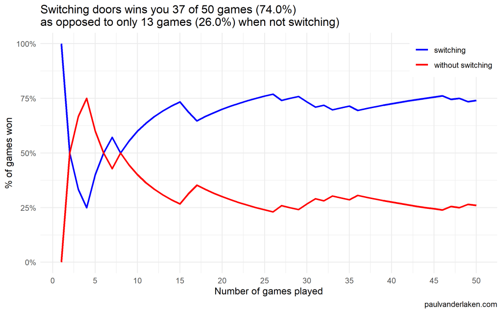
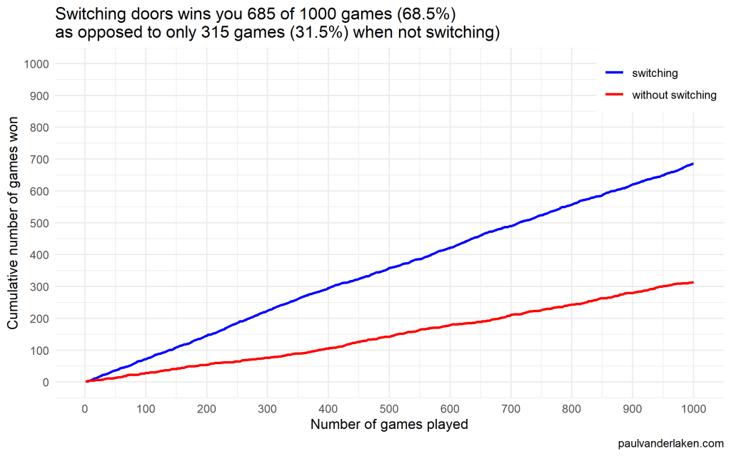
Visualizations (ggplot2)
I specifically picked a seed (the second one I tried) in which not switching looked like it was better during the first few games played.
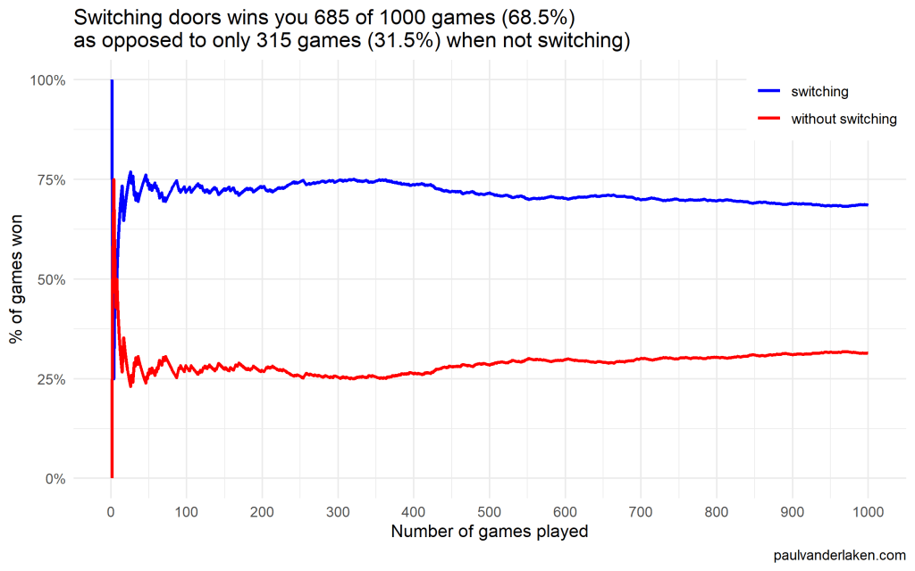
In R, I made an additional plot that shows the probabilities converging.
As we play more and more games, our results move to the actual probabilities of winning:
After the first four games, you could have erroneously concluded that not switching would result in better chances of you winning a sports car. However, in the long run, that is definitely not true.
I was actually suprised to see that these lines look to be mirroring each other. But actually, that’s quite logical maybe… We already had the car with our initial door guess in those games. If we would have sticked to that initial choice of a door, we would have won, whereas all the cases where we switched, we lost.
Keep me posted!
I hope you enjoyed these simulations and visualizations, and am curious to see what you come up with yourself!
For instance, you could increase the number of doors in the game, or the number of goat-doors Monty Hall opens. When does it become a disadvantage to switch?
I don’t want to participate in the general debate on COVID19 as there are enough, much more knowledgeable experts doing so already.
However, I did want to share something that sparked my interest: this great article by the Washington Post where they show the importance of social distancing in case of viral outbreaks with four simple simulations:
Regular viral outbreak
Viral outbreak with forced (temporary) quarantaine
Viral outbreak with moderate social distancing
Viral outbreak with extensive social distancing
While these are obviously much oversimplified models of reality, the results convey a powerful and very visual message showing the importance of our social behavior in such a crisis.
1. Simulation of regular viral outbreak2. Simulation with temporary quarantaine opening up.
Bayesian networks are a type of probabilistic graphical model that uses Bayesian inference for probability computations. Bayesian networks aim to model conditional dependence, and therefore causation, by representing conditional dependence by edges in a directed graph. Through these relationships, one can efficiently conduct inference on the random variables in the graph through the use of factors.
As Bayes nets represent data as a probabilistic graph, it is very easy to use that structure to simulate new data that demonstrate the realistic patterns of the underlying causal system. Daniel’s post shows how to do this with bnlearn.
Daniel’s example Bayes net
New data is simulated from a Bayes net (see above) by first sampling from each of the root nodes, in this case sex. Then followed by the children conditional on their parent(s) (e.g. sport | sex and hg | sex) until data for all nodes has been drawn. The numbers on the nodes below indicate the sequence in which the data is simulated, noting that rcc is the terminal node.
The original and simulated datasets are compared in a couple of ways 1) observing the distributions of the variables 2) comparing the output from various models and 3) comparing conditional probability queries. The third test is more of a sanity check. If the data is generated from the original Bayes net then a new one fit on the simulated data should be approximately the same. The more rows we generate the closer the parameters will be to the original values.
The original data alongside the generated data in Daniel’s example
As you can see, a Bayesian network allows you to generate data that looks, feels, and behaves a lot like the data on which you based your network on in the first place.
This can be super useful if you want to generate a synthetic / fake / artificial dataset without sharing personal or sensitive data.
Moreover, the underlying Bayesian net can be very useful to compute missing values. In Daniel’s example, he left out some values on purpose (pretending they were missing) and imputed them with the Bayes net. He found that the imputed values for the missing data points were quite close to the original ones:
For two variables, the original values plotted against the imputed replacements.
In the original blog, Daniel goes on to show how to further check the integrity of the simulated data using statistical models and shares all his code so you can try this out yourself. Please do give his website a visit as Daniel has many more interesting statistics blogs!
We can’t just throw data into machines and expect to see any meaning […], we need to think [about this]. I see a strong trend in the practitioners community to just automate everything, to just throw data into a black box and expect to get money out of it, and I really don’t believe in that.
All pictures below are slides from the above video.
My summary / interpretation
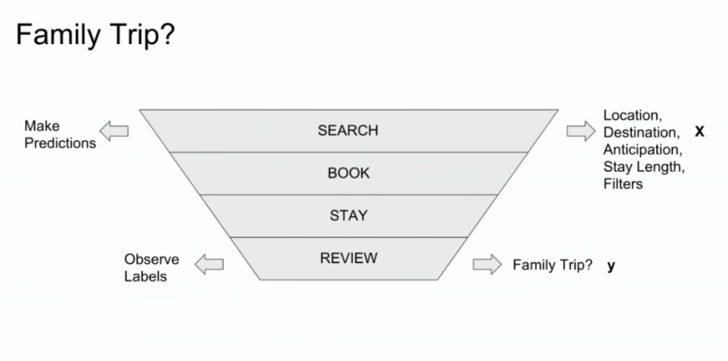
Lucas highlights an example he has been working on at Booking.com, where they seek to predict which searching activities on their website are for family trips.
What happens is that people forget to specify that they intend to travel as a family, forget to input one/two/three child travellers will come along on the trip, and end up not being able to book the accomodations that come up during their search. If Booking.com would know, in advance, that people (may) be searching for family accomodations, they can better guide these bookers to family arrangements.
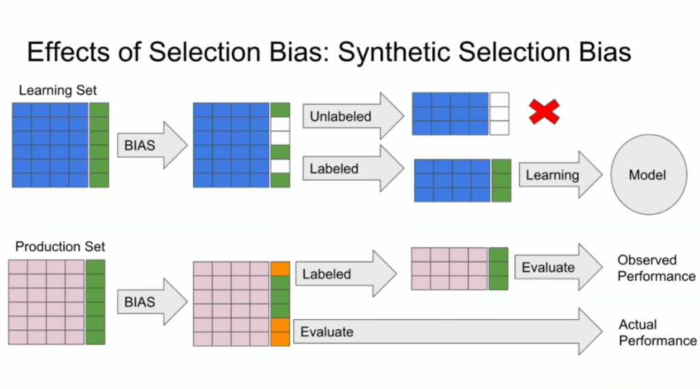
The problem here is that many business processes in real life look and act like a funnel. Samples drop out of the process during the course of it. So too the user search activity on Booking.com’s website acts like a funnel.
People come to search for arrangements
Less people end up actually booking arrangements
Even less people actually go on their trip
And even less people then write up a review
However, only for those people that end up writing a review, Booking.com knows 100% certain that they it concerned a family trip, as that is the moment the user can specify so. Of all other people, who did not reach stage 4 of the funnel, Booking.com has no (or not as accurate an) idea whether they were looking for family trips.
Such a funnel thus inherently produces business data with selection bias in it. Only for people making it to the review stage we know whether they were family trips or not. And only those labeled data can be used to train our machine learning model.
And now for the issue: if you train and evaluate a machine learning model on data generated with such a selection bias, your observed performance metrics will not reflect the actual performance of your machine learning model!
Actually, they are pretty much overestimates.
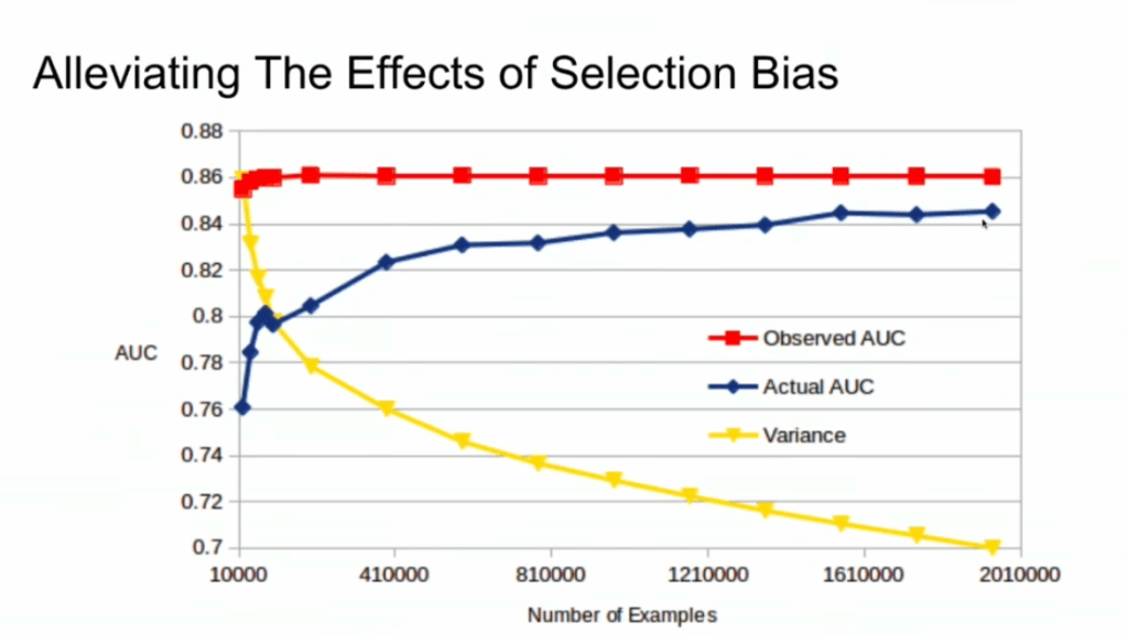
This is very much an issue, even though many ML practitioners don’t see aware. Selection bias makes us blind as to the real performance of our machine learning models. It produces high variance in the region of our feature space where labels are missing. This leads us to being overconfident in our ability to predict whether some user is looking for a family trip. And if the mechanism causing the selection bias is still there, we could never find out that we are overconfident. Consistently estimating, say, 30% of people are looking for family trips, whereas only 25% are.
Fortunately, Lucas proposes a very simple solution! Just adding more observations can (partially) alleviate this detrimental effect of selection bias. Although our bias still remains, the variance goes down and the difference between our observed and actual performance decreases.
A second issue and solution to selection bias relates to propensity (see also): the extent to which your features X influence not only the outcome Y, but also the selection criteria s.
If our features X influence both the outcome Y but also the selection criteria s, selection bias will occur in your data and can thus screw up your conclusion. In order to inspect to what extent this occurs in your setting, you will want to estimate a propensity model. If that model is good, and X appears valuable in predicting s, you have a selection bias problem.
Via a propensity model s ~ X, we quantify to what extent selection bias influences our data and model. The nice thing is that we, as data scientists, control the features X we use to train a model. Hence, we could just use only features X that do not predict s to predict Y. Conclusion: we can conduct propensity-based feature selection in our Y ~ X by simply avoiding features X that predicted s!
Still, Lucas does point that this becomes difficult when you have valuable features that predict both s and Y. Hence, propensity-based feature selection may end up cost(ing) you performance, as you will need to remove features relevant to Y.