Tag: visual

Making GIFs with Processing

Processing is a flexible software sketchbook and a language for learning how to code within the context of the visual arts. It’s open-source, there are many online materials, and the language itself is very accessible.

I recently stumbled upon 17-year-old Joseff Nic from Cardiff who has been making GIFs in Processing only since 2018, but which are turning out fantastic already. You can hire him here, and have a look at his Twitter, Tumbler or Drimble channels for the originals:

#processing pic.twitter.com/ENcGeUihHx
— Jo (@jn3008) September 15, 2019

Here are some more of Joseff’s creations:

Wave Swirl loop design processing gif animation

Some of Joseff’s work seems inspired by David Whyte, a graphic designer from Ireland. His portfolio is quite impressive as well, very visually pleasing, and you can hire him here.

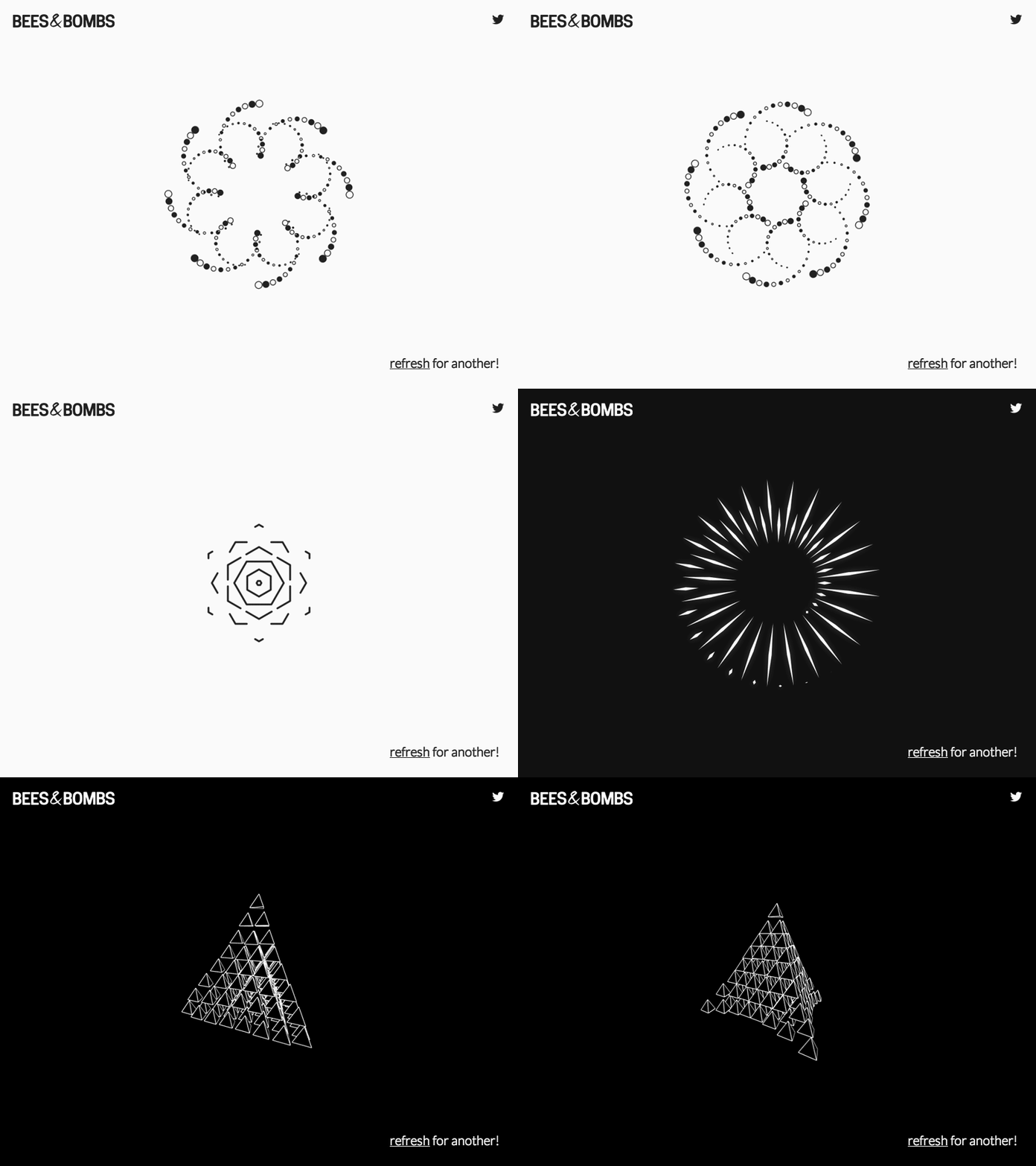
Bees & Bombs Roulette gif processing web web design

StudioPhi spiral gif processing geometry motion

Knot geometry motion design processing gif

If you’re interesting in learning Processing, Daniel Shiffman demonstrates how to create the most amazing things in Processing via his Youtube channel the Coding Train, which I’ve covered before.

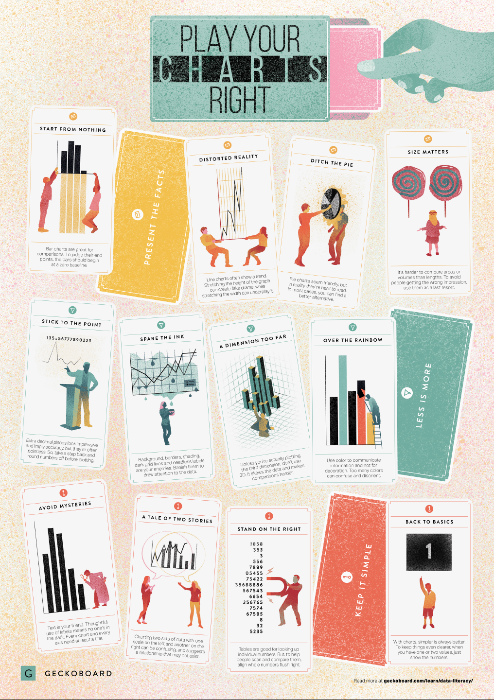
Play Your Charts Right: Tips for Effective Data Visualization – by Geckoboard

In a world where data really matters, we all want to create effective charts. But data visualization is rarely taught in schools, or covered in on-the-job training. Most of us learn as we go along, and therefore we often make choices or mistakes that confuse and disorient our audience.
From overcomplicating or overdressing our charts, to conveying an entirely inaccurate message, there are common design pitfalls that can easily be avoided. We’ve put together these pointers to help you create simpler charts that effectively get across the meaning of your data.
Geckoboard

Based on work by experts such as Stephen Few, Dona Wong, Albert Cairo, Cole Nussbaumer Knaflic, and Andy Kirk, the authors at Geckoboard wrote down a list of recommendations which I summarize below:

Present the facts

Start your axis at zero whenever possible, to prevent misinterpretation. Particularly bar charts.
The width and height of line and scatter plots influence its messages.
Area and size are hard to interpret. Hence, there’s often a better alternative to the pie chart. Read also this.

Via Geckoboard
Via Geckoboard

Less is more

Use colors for communication, not decoration.
Diminish non-data ink, to draw attention to that which matters.
Do not use the third dimension, unless you are plotting it.
Avoid overselling numerical accuracy with precise decimal values.

Via Geckoboard
Via Geckoboard

Keep it simple

Annotate your plots; include titles, labels or scales.
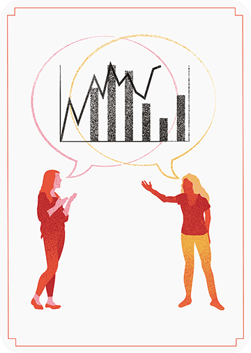
Avoid squeezing too much information in a small space. For example, avoid a second x- or y-axis whenever possible.
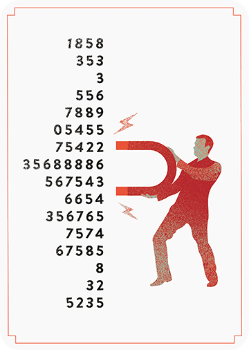
Align your numbers right, literally.
Don’t go for fancy; go for clear. If you have few values, just display the values.

Via Geckoboard
Via Geckoboard

Infographic summary

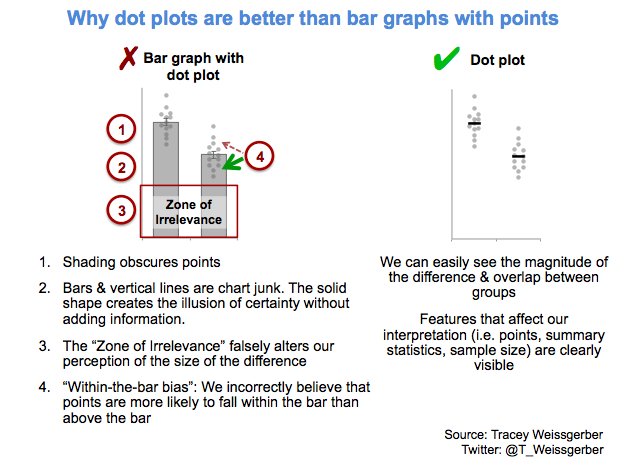
Avoid bar plots for continuous data! Do this instead:

Tracey Weissgerber, Natasa Milic, Stacey Winham, and Vesna Garovic wrote this interesting 2015 paper on bar graphs. By a systematic review of physiology research, they demonstrate we need to reconsider how we present continuous data in small samples.

Bar and line plots are commonly used to display continuous data. This is problematic, as many different data distributions can lead to the same bar or line graph. Nevertheless, the rarely used scatterplots, box plots, and histograms much better allow users to critically evaluate continuous data.

They provide many interesting visuals that underline their argument.

For instance, the four datasets below (B, C, D, and E) will all result in the same barplot (A), whereas they demonstrate quite different characteristics.

Alternatively, bar plots are often used for to display group means when observations within groups may not be independent. For instance, it could be that the bars below represent two measurement occassians, and that each of our sampled observations occurs in both. In that case, the scatterplots with connected dots may be more suitable. While the bars in plot A would represent datasets B, C, and D, these are clearly different when viewed in scatterplots.

Also, a lot of meaningful information is typically lost in bar plots. For instance, the number of observations in a group. But also the distribution of values. While the former can be added (see B below), the latter can much better be shown in a scatter plot like C (below).

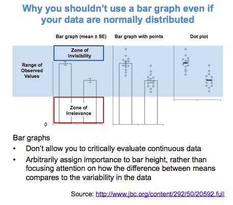
Actually, in a later blog post, lead researcher Tracey Weissgerber shares the below visual. It highlights the distractive irrelevance of bar plot and the information that is lost (becomes invisible) when opting for a bar chart.

Tracey refactored this into a similar visual of her own:

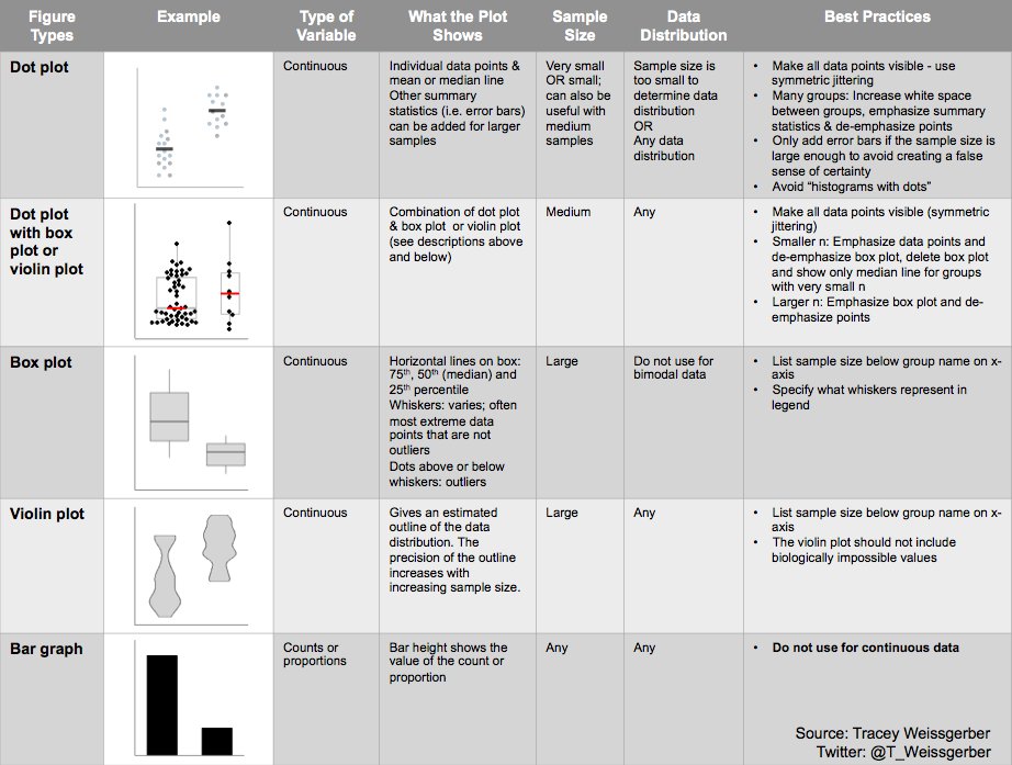
So what can you do instead, you may ask yourself. To this question too, Tracey has an answer, sharing the below overview of alternatives options:

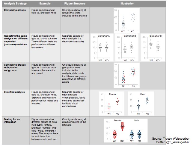
She made another overview which may help you pick the best visual for your data. This one takes your intention behind the visual as a starting point, though is unfortunately a bit low quality:

Chatterplots

I’ve mentioned before that I dislike wordclouds (for instance here, or here) and apparently others share that sentiment. In his recent Medium blog, Daniel McNichol goes as far as to refer to the wordcloud as the pie chart of text data! Among others, Daniel calls wordclouds disorienting, one-dimensional, arbitrary and opaque and he mentions their lack of order, information, and scale.

Wordcloud of the negative characteristics of wordclouds, via Medium

Instead of using wordclouds, Daniel suggests we revert to alternative approaches. For instance, in their Tidy Text Mining with R book, Julia Silge and David Robinson suggest using bar charts or network graphs, providing the necessary R code. Another alternative is provided in Daniel’s blog: the chatterplot!

While Daniel didn’t invent this unorthodox wordcloud-like plot, he might have been the first to name it a chatterplot. Daniel’s chatterplot uses a full x/y cartesian plane, turning the usually only arbitrary though exploratory wordcloud into a more quantitatively sound, information-rich visualization.

R package ggplot’s geom_text() function — or alternatively ggrepel‘s geom_text_repel() for better legibility — is perfectly suited for making a chatterplot. And interesting features/variables for the axis — apart from the regular word frequencies — can be easily computed using the R tidytext package.

Here’s an example generated by Daniel, plotting words simulatenously by their frequency of occurance in comments to Hacker News articles (y-axis) as well as by the respective popularity of the comments the word was used in (log of the ranking, on the x-axis).

[CHATTERPLOTs are] like a wordcloud, except there’s actual quantitative logic to the order, placement & aesthetic aspects of the elements, along with an explicit scale reference for each. This allows us to represent more, multidimensional information in the plot, & provides the viewer with a coherent visual logic& direction by which to explore the data.
Daniel McNichol via Medium

I highly recommend the use of these chatterplots over their less-informative wordcloud counterpart, and strongly suggest you read Daniel’s original blog, in which you can also find the R code for the above visualizations.

Add a self-explantory legend to your ggplot2 boxplots

Laura DeCicco found that non-R users keep asking her what her box plots exactly mean or demonstrate. In a recent blog post, she therefore breaks down the calculations into easy-to-follow chunks of code. Even better, she included the source code to make boxplots that come with a very elaborate default legend:

As you can see, the above contains much more and easier to understand information than the original ggplot2 boxplot below.

Laura wrote the custom function ggplot_box_legend() (see source code below and in Laura’s blog), which uses the cowplot package to paste the explanation to the box plot. All you need to do is call the legend function just before you run your ggplot2 boxplot call.

ggplot_box_legend <- function(family = "serif"){
  
  # Create data to use in the boxplot legend:
  set.seed(100)

  sample_df <- data.frame(parameter = "test",
                        values = sample(500))

  # Extend the top whisker a bit:
  sample_df$values[1:100] <- 701:800
  # Make sure there's only 1 lower outlier:
  sample_df$values[1] <- -350
  
  # Function to calculate important values:
  ggplot2_boxplot <- function(x){
  
    quartiles <- as.numeric(quantile(x, 
                                     probs = c(0.25, 0.5, 0.75)))
    
    names(quartiles) <- c("25th percentile", 
                          "50th percentile\n(median)",
                          "75th percentile")
    
    IQR <- diff(quartiles[c(1,3)])
  
    upper_whisker <- max(x[x < (quartiles[3] + 1.5 * IQR)])
    lower_whisker <- min(x[x > (quartiles[1] - 1.5 * IQR)])
      
    upper_dots <- x[x > (quartiles[3] + 1.5*IQR)]
    lower_dots <- x[x < (quartiles[1] - 1.5*IQR)]
  
    return(list("quartiles" = quartiles,
                "25th percentile" = as.numeric(quartiles[1]),
                "50th percentile\n(median)" = as.numeric(quartiles[2]),
                "75th percentile" = as.numeric(quartiles[3]),
                "IQR" = IQR,
                "upper_whisker" = upper_whisker,
                "lower_whisker" = lower_whisker,
                "upper_dots" = upper_dots,
                "lower_dots" = lower_dots))
  }
  
  # Get those values:
  ggplot_output <- ggplot2_boxplot(sample_df$values)
  
  # Lots of text in the legend, make it smaller and consistent font:
  update_geom_defaults("text", 
                     list(size = 3, 
                          hjust = 0,
                          family = family))
  # Labels don't inherit text:
  update_geom_defaults("label", 
                     list(size = 3, 
                          hjust = 0,
                          family = family))
  
  # Create the legend:
  # The main elements of the plot (the boxplot, error bars, and count)
  # are the easy part.
  # The text describing each of those takes a lot of fiddling to
  # get the location and style just right:
  explain_plot <- ggplot() +     stat_boxplot(data = sample_df,                  aes(x = parameter, y=values),                  geom ='errorbar', width = 0.3) +     geom_boxplot(data = sample_df,                  aes(x = parameter, y=values),                   width = 0.3, fill = "lightgrey") +     geom_text(aes(x = 1, y = 950, label = "500"), hjust = 0.5) +     geom_text(aes(x = 1.17, y = 950,                   label = "Number of values"),               fontface = "bold", vjust = 0.4) +     theme_minimal(base_size = 5, base_family = family) +     geom_segment(aes(x = 2.3, xend = 2.3,                       y = ggplot_output[["25th percentile"]],                       yend = ggplot_output[["75th percentile"]])) +     geom_segment(aes(x = 1.2, xend = 2.3,                       y = ggplot_output[["25th percentile"]],                       yend = ggplot_output[["25th percentile"]])) +     geom_segment(aes(x = 1.2, xend = 2.3,                       y = ggplot_output[["75th percentile"]],                       yend = ggplot_output[["75th percentile"]])) +     geom_text(aes(x = 2.4, y = ggplot_output[["50th percentile\n(median)"]]),                label = "Interquartile\nrange", fontface = "bold",               vjust = 0.4) +     geom_text(aes(x = c(1.17,1.17),                    y = c(ggplot_output[["upper_whisker"]],                         ggplot_output[["lower_whisker"]]),                    label = c("Largest value within 1.5 times\ninterquartile range above\n75th percentile",                             "Smallest value within 1.5 times\ninterquartile range below\n25th percentile")),                   fontface = "bold", vjust = 0.9) +     geom_text(aes(x = c(1.17),                    y =  ggplot_output[["lower_dots"]],                    label = "Outside value"),                vjust = 0.5, fontface = "bold") +     geom_text(aes(x = c(1.9),                    y =  ggplot_output[["lower_dots"]],                    label = "-Value is >1.5 times and"), 
              vjust = 0.5) +
    geom_text(aes(x = 1.17, 
                  y = ggplot_output[["lower_dots"]], 
                  label = "<3 times the interquartile range\nbeyond either end of the box"), 
              vjust = 1.5) +
    geom_label(aes(x = 1.17, y = ggplot_output[["quartiles"]], 
                  label = names(ggplot_output[["quartiles"]])),
              vjust = c(0.4,0.85,0.4), 
              fill = "white", label.size = 0) +
    ylab("") + xlab("") +
    theme(axis.text = element_blank(),
          axis.ticks = element_blank(),
          panel.grid = element_blank(),
          aspect.ratio = 4/3,
          plot.title = element_text(hjust = 0.5, size = 10)) +
    coord_cartesian(xlim = c(1.4,3.1), ylim = c(-600, 900)) +
    labs(title = "EXPLANATION")

  return(explain_plot) 
  
}

ggplot_box_legend()

What to consider when choosing colors for data visualization, by DataWrapper.de

Lisa Charlotte Rost of DataWrapper often writes about data visualization and lately she has focused on the (im)proper use of color in visualization. In this recent blog, she gives a bunch of great tips and best practices, some of which I copied below: