For fresh R programmers, vectorization can sound awfully complicated. Consider two math problems, one vectorized, and one not:
Two ways of doing the same computations in R
Why on earth should R spend more time calculating one over the other? In both cases there are the same three addition operations to perform, so why the difference? This is what we will try to illustrate in this post, which is inspired on work by Naom Ross and the University of Auckland.
R behind the scenes:
R is a high-level, interpreted computer language. This means that R takes care of a lot of basic computer tasks for you. For instance, when you type i <- 5.0 you don’t have to tell R:
That 5.0 is a floating-point number
That i should store numeric-type data
To find a place in memory for to put 5
To register i as a pointer to that place in memory
You also don’t have to convert i <- 5.0 to binary code. That’s done automatically when you hit Enter. Although you are probably not aware of this, many R functions are just wrapping your input and passing it to functions of other, compiled computer languages, like C, C++, or FORTRAN, in the back end.
Now here’s the crux: If you need to run a function over a set of values, you can either pass in a vector of these values through the R function to the compiled code (math example 1), or you could call the R function repeatedly for each value separately (math example 2). If you do the latter, R has to do stuff (figuring out the above bullet points and translating the code) each time, repeatedly. However, if you call the function with a vector instead, this figuring out part only happens once. For instance, R vectors are constricted to a single data type (e.g., numeric, character) and when you use a vector instead of seperate values, R only needs to determine the input data type once, which saves time. In short, there’s no advantage to NOT organizing your data as vector.
For-loops and functional programming (*ply)
One example of how new R programmers frequently waste computing time is via memory allocation. Take the below for loop, for instance:
iterations = 10000000

 system.time({
   j = c()
   for(i in 1:iterations){
     j[i] <- i
   }
 })
##    user  system elapsed
##    3.71    0.23    3.94
Here, vector j starts out with length 1, but for each iteration in the for loop, R has to re-size the vector and re-allocate memory. Recursively, R has to find the vector in its memory, create a new vector that will fit more data, copy the old data over, insert the new data, and erase the old vector. This process gets very slow as vectors get big. Nevertheless, it is often how programmers store the results of their iterative processes. Tremendous computing power can be saved by pre-allocating vectors to fit all the values beforehand, so that R does not have to do unnecessary actions:
system.time({
   j = rep(NA, iterations)
   for(i in 1:iterations){
     j[i] <- i
   }
 })
##    user  system elapsed
##    0.88    0.01    0.89
More advanced R users tend to further optimize via functionals. This family of functions takes in vectors (or matrices, or lists) of values and applies other functions to each. Examples are apply or plyr::*ply functions, which speed up R code mainly because the for loops they have inside them automatically do things like pre-allocating vector size. Functionals additionally prevent side effects: unwanted changes to your working environment, such as the remaining i after for(i in 1:10). Although this does not necessarily improve computing time, it is regarded best practice due to preventing consequent coding errors.
Conclusions
There are cases when you should use for loops. For example, the performance penalty for using a for loop instead a vector will be small if the number of iterations is relatively small, and the functions called inside your for loop are slow. Here, looping and overhead from function calls make up a small fraction of your computational time and for loops may be more intuitive or easier to read for you. Additionally, there are cases where for loops make more sense than vectorized functions: (1) when the functions you seek to apply don’t take vector arguments and (2) when each iteration is dependent on the results of previous iterations.
Another general rule: fast R code is short. If you can express what you want to do in R in a line or two, with just a few function calls that are actually calling compiled code, it’ll be more efficient than if you write long program, with the added overhead of many function calls.
Finally, there is a saying that “premature optimization is the root of all evil”. What this means is that you should not re-write your R code unless the computing time you are going to save is worth the time invested. Nevertheless, if you understand how vectorization and functional programming work, you will be able to write more faster, safer, and more transparent (short & simple) programs.
Reinforcement learning is an area of machine learning inspired by behavioral psychology, concerned with how software agents ought to take actions in an environment so as to maximize some notion of cumulative reward (Wikipedia, 2017). Normally, reinforcement learning occurs autonomously. Here, algorithms will seek to minimize/maximize a score that is estimated via predefined constraints. As such, algorithms can thus learn to perform the most effective actions (those that minimize/maximize the score) by repeatedly experimenting and assessing strategies.
The approach in the video below is radically different. Instead of a pre-defined scoring, human-computer interaction is used to assign each action sequence (each iteration/experiment) a score. This approach is particularly useful for complex behaviors, such as a back-flip, for which it is hard to pre-define the constraints and actions that lead to the “most effective” back-flip. However, for us humans, it is relatively easy to recognize a good back-flip when we see one. The video below shows how the researchers therefore integrated a human-computer interaction in their reinforcement learning algorithm. After observing the algorithm perform a sequence of actions, a human actor indicates to what extent the goal (i.e., a backflip) is achieved or not. This human assessment thus functions as the score which the algorithm will try to minimize/maximize.
This approach can be really valuable for organizations seeking to improve their machine learning application. The paper on the principle (Deep Reinforcement Learning from Human Preferences) can be found here. The scholars conclude that this supervised approach based on human preferences has very good training results whereas the cost are similar the simple bulldozer approach of training a neural net from scratch using GPU servers.
The Deep Learning textbook helps students and practitioners enter the field of machine learning in general and deep learning in particular. Its online version is available online for free whereas a hardcover copy can be ordered here on Amazon. You can click on the topics below to be redirected to the book chapter:
The following is the first part of my introduction to regular expression (regex), in general, and the use of regex in R, in specific. It is loosely inspired on the swirl() tutorial by Jon Calder. I created it in R Markdown and uploaded it to RPubs, for an easier read.
Regular expression
A regular expression, regex or regexp (sometimes called a rational expression) is, in theoretical computer science and formal language theory, a sequence of characters that define a search pattern. Usually this pattern is then used by string searching algorithms for “find” or “find and replace” operations on strings (Wikipedia). Regular expressions were originally developed for the Perl language and have since been implemented in many other languages including R.
Regular expressions usually involve two parts: a pattern and a text string. The pattern defines what type and/or sequence of characters to look for whereas the text string represents the content in which to search/match this pattern. Patterns are always strings themselves and thus need to be enclosed in (single or double) quotation marks.
Example
An example: the pattern “stat” will match the occurance of the letters “s”, “t”, “a”, “t” in that specific order. Regardless of where in the content (text string) they occur and what other characters may precede the “s” or follow the last “t”.
Base R’s grepl() function returns a logical value reflecting whether the pattern is matched. The below demonstrates how the pattern “stats” can be found in both “statistics” and “estate” but not in “castrate” (which does include the letters, but with an r in between), in “catalyst” (which does include the letters, but not in the right order), or in “banana” (which does not include all the letters).
Moreover, regular expressions are case sensitive, so “stat” is not found in “Statistics”, unless it is specified that case should be ignored (FALSE by default).
Base R includes seven main functions that use regular expressions with different outcomes. These are grep(), grepl(), regexpr(), gregexpr(), regexec(), sub(), and gsub(). Although they require mostly similar inputs, their returned values are quite different.
grep() & grepl()
grep() examines each element of a character vector and returns the indices where the pattern is matched.
sentences=c("I like statistics", "I like bananas", "Estates and statues are expensive")grep("stat", sentences)
## [1] 1 3
By setting the value parameter to TRUE, grep() will return the character element instead of its index.
grep("stat", sentences, value=TRUE)
## [1] "I like statistics" "Estates and statues are expensive"
It’s logical brother grepl() you’ve seen before. It returns a logical value instead of the index or the element.
grepl("stat", sentences)
## [1] TRUE FALSE TRUE
regexpr() & gregexpr()
regexpr() seeks for a pattern in a text and returns an integer vector with two attributes (also vectors). The main integer vector returned represents the position where the pattern was first matched in the text. Its attribute “match.length” is also an integer vector representing the length of the match (in this case “stat” is always length 4).
If the pattern is not matched, both of the main vector and the length attribute will have a value of -1.
The second attribute (“useBytes”) is always a logical vector of length one. It represents whether matching is done byte-by-byte (TRUE) or character-by-character (FALSE), but you may disregard it for now.
sentences
## [1] "I like statistics"                 "I like bananas"
## [3] "Estates and statues are expensive"
Note that, for the third sentence, regexpr() only returns the values for the first match (i.e., “Estate”) but not those of the second match (i.e., “statues”). For this reason, the function has a brother, gregexpr(), which has the same functionality but performs the matching on a global scale (hence the leading g). This means that the algorithm does not stop after its first match, but continues and reports all matches within the content string.
grepexpr() thus does not return a single vector, but a list of vectors. Each of these vectors reflects an input content string as is the length of the number of matches within that content. For example, the “stat” pattern is matched twice in our third sentence, therefore its vector is length 2, with the starting position of each match as well as their lengths.
sentences
## [1] "I like statistics"                 "I like bananas"
## [3] "Estates and statues are expensive"
In order to explain how regexec() differs from gregexpr(), we first need to explain how parentheses in work in regex. Most simply speaking, parentheses or round brackets (()) indicate groups. One of the advantages of groups is that logical tests can thus be conducted within regular expressions.
sentences
## [1] "I like statistics"                 "I like bananas"
## [3] "Estates and statues are expensive"
grepl("like", sentences)
## [1] TRUE TRUE FALSE
grepl("are", sentences)
## [1] FALSE FALSE TRUE
grepl("(are|like)", sentences)
## [1] TRUE TRUE TRUE
regexec()
However, these groups can also be useful to extract more detailed information from a regular expression. This is where regexec() comes in.
Like gregexpr(), regexec() returns a list of the same length as the content. This list includes vectors that reflect the starting positions of the overall match, as well as the matches corresponding to parenthesized subpatterns. Similarly, attribute “match.length” reflects the lengths of each of the overall and submatches. In case no match is found, a -1 value is again returned.
The beauty of regexec() because clear when we split our pattern into two groups using parentheses: “(st)(at)”. As you can see below, both regexpr() and its global brother gregexpr() disregard this grouping and provide the same output as before – as you would expect for the pattern “stat”. In contast, regexec() notes that we now have a global pattern (“stat”)as well as two subpatterns (“st” and “at”). For each of these, the function returns the starting positions as well as the pattern lengths.
sentences
## [1] "I like statistics"                 "I like bananas"
## [3] "Estates and statues are expensive"
The final two base regex functions are sub() and its global brother gsub(). These, very intiutively, substitute a matched pattern by a specified replacement and then return all inputs. For instance, we could replace “I” with “You” in our example sentences.
sub(pattern="I", replacement="You", sentences)
## [1] "You like statistics"               "You like bananas"
## [3] "Estates and statues are expensive"
Similarly, we could desire to replace all spaces by underscores. This would require a global search (i.e., gsub()), as sub() would stop after the first match.
This was the first part of my introduction to Regular Expression in R. For more information detailed information about all input parameters of each function, please consult the base R manual. In subsequent parts, I will introduce you to so-called Anchors, Character Classes, Groups, Ranges, and Quantifiers. These will allow you to perform more advanced searches and matches. Here, we will also elaborate on lazy, greedy, and possesive regular expressions, which further expand our search capability as well as flexibility.
In the end, I hope to provide you with an overview of several Regular Expressions that I have found extremely useful in my personal project, and which should be valuable to anyone who conducts applied research (in organizations).
Simpson (1951) demonstrated that a statistical relationship observed within a population—i.e., a group of individuals—could be reversed within all subgroups that make up that population. This phenomenon, where X seems to relate to Y in a certain way, but flips direction when the population is split for W, has since been referred to as Simpson’s paradox. Others names, according to Wikipedia, include the Simpson-Yule effect, reversal paradox or amalgamation paradox.
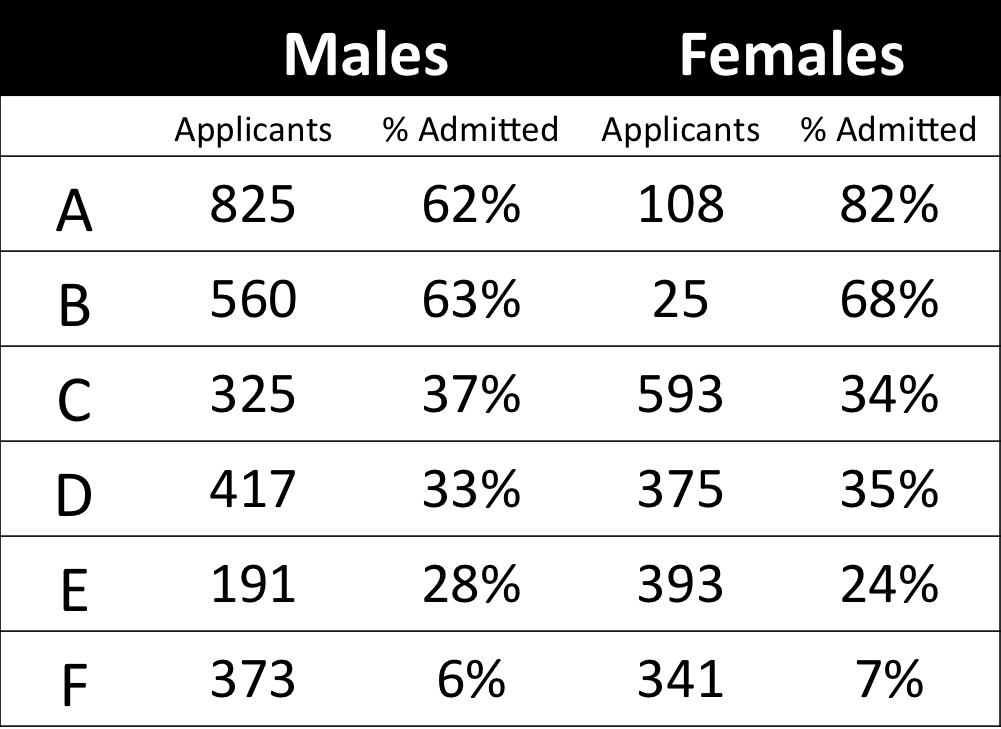
The most famous example has to be the seemingly gender-biased Berkeley admission rates:
“Examination of aggregate data on graduate admissions to the University of California, Berkeley, for fall 1973 shows a clear but misleading pattern of bias against female applicants. Examination of the disaggregated data reveals few decision-making units that show statistically significant departures from expected frequencies of female admissions, and about as many units appear to favor women as to favor men. If the data are properly pooled, taking into account the autonomy of departmental decision making, thus correcting for the tendency of women to apply to graduate departments that are more difficult for applicants of either sex to enter, there is a small but statistically significant bias in favor of women. […] The bias in the aggregated data stems not from any pattern of discrimination on the part of admissions committees, which seem quite fair on the whole, but apparently from prior screening at earlier levels of the educational system.” – part of abstract of Bickel, Hammel, & O’Connel (1975)
In a table, the effect becomes clear. While it seems as if women are rejected more often overall, women are actually less often rejected on a departmental level. Women simply applied to more selective departments more often (E & C below), resulting in the overall lower admission rate for women (35% as opposed to 44% for men).
Simpsons Paradox can easily occur in organizational or human resources settings as well. Let me run you through two illustrated examples, I simulated:
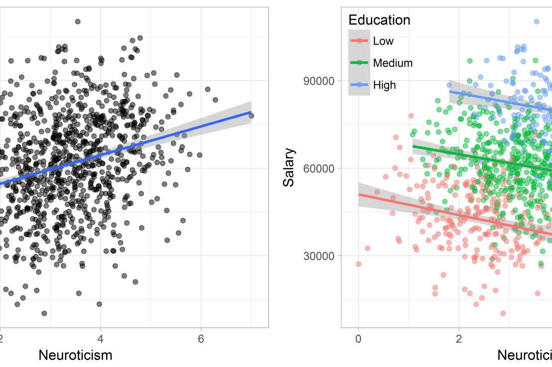
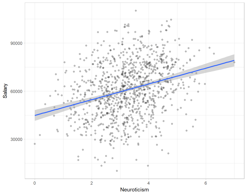
Assume you run a company of 1000 employees and you have asked all of them to fill out a Big Five personality survey. Per individual, you therefore have a score depicting his/her personality characteristic Neuroticism, which can run from 0 (not at all neurotic) to 7 (very neurotic). Now you are interested in the extent to which this Neuroticism of employees relates to their Job Performance (measured 0 – 100) and their Salary (measured in Euro’s per Year). In order to get a sense of the effects, you may decide to visualize both these relations in scatter plots:
From these visualizations it would look like Neuroticism relates significantly and positively to both employees’ performance and their yearly salary. Should you select more neurotic people to improve your overall company performance? Or are you discriminating emotionally-stable (non-neurotic) employees when it comes to salary?
Taking a closer look at the subgroups in your data, you might however find very different relationships. For instance, the positive relationship between neuroticism and performance may only apply to technical positions, but not to those employees’ in service-oriented jobs.
Similarly, splitting the employees by education level, it becomes clear that there is a relationship between neuroticism and education level that may explain the earlier association with salary. More educated employees receive higher salaries and within these groups, neuroticism is actually related to lower yearly income.
If you’d like to see the code used to simulate these data and generate the examples, you can find the R markdown file here on Rpubs.
Solving the paradox
Kievit and colleagues (2013) argue that Simpsons paradox may occur in a wide variety of research designs, methods, and questions, particularly within the social and medical sciences. As such, they propose several means to “control” or minimize the risk of it occurring. The paradox may be prevented from occurring altogether by more rigorous research design: testing mechanisms in longitudinal or intervention studies. However, this is not always feasible. Alternatively, the researchers pose that data visualization may help recognize the patterns and subgroups and thereby diagnose paradoxes. This may be easy if your data looks like this:
But rather hard, or even impossible, when your data looks more like the below:
Clustering may nevertheless help to detect Simpson’s paradox when it is not directly observable in the data. To this end, Kievit and Epskamp (2012) have developed a tool to facilitate the detection of hitherto undetected patterns of association in existing datasets. It is written in R, a language specifically tailored for a wide variety of statistical analyses which makes it very suitable for integration into the regular analysis workflow. As an R package, the tool is is freely available and specializes in the detection of cases of Simpson’s paradox for bivariate continuous data with categorical grouping variables (also known as Robinson’s paradox), a very common inference type for psychologists. Finally, its code is open source and can be extended and improved upon depending on the nature of the data being studied.
One example of application is provided in the paper, for a dataset on coffee and neuroticism. A regression analysis would suggest a significant positive association between coffee and neuroticism overall. However, when the detection algorithm of the R package is applied, a different picture appears: the analysis shows that there are three latent clusters present and that the purported positive relationship only holds for one cluster whereas it is negative in the others.
Update 24-10-2017: minutephysics – one of my favorite YouTube channels – uploaded a video explaining Simpson’s paradox very intuitively in a medical context:
Update 01-11-2017: minutephysics uploaded a follow-up video:
The paradox is that we remain reluctant to fight our bias, even when they are put in plain sight.


