Category: visualization

Visualizing model uncertainty

ungeviz is a new R package by Claus Wilke, whom you may know from his amazing work and books on Data Visualization. The package name comes from the German word “Ungewissheit”, which means uncertainty. You can install the developmental version via:

devtools::install_github("clauswilke/ungeviz")

The package includes some bootstrapping functionality that, when combined with ggplot2 and gganimate, can produce some seriousy powerful visualizations. For instance, take the below piece of code:

data(BlueJays, package = "Stat2Data")

# set up bootstrapping object that generates 20 bootstraps
# and groups by variable `KnownSex`
bs <- ungeviz::bootstrapper(20, KnownSex)

ggplot(BlueJays, aes(BillLength, Head, color = KnownSex)) +
  geom_smooth(method = "lm", color = NA) +
  geom_point(alpha = 0.3) +
  # `.row` is a generated column providing a unique row number
  # to all rows in the bootstrapped data frame 
  geom_point(data = bs, aes(group = .row)) +
  geom_smooth(data = bs, method = "lm", fullrange = TRUE, se = FALSE) +
  facet_wrap(~KnownSex, scales = "free_x") +
  scale_color_manual(values = c(F = "#D55E00", M = "#0072B2"), guide = "none") +
  theme_bw() +
  transition_states(.draw, 1, 1) + 
  enter_fade() + 
  exit_fade()

Here’s what’s happening:

Claus loads in the BlueJays dataset, which contains some data on birds.
He then runs the ungezviz::bootstrapper function to generate a new dataset of bootstrapped samples.
Next, Claus uses ggplot2::geom_smooth(method = "lm") to run a linear model on the orginal BlueJays dataset, but does not color in the regression line (color = NA), thus showing only the confidence interval of the model.
Moreover, Claus uses ggplot2::geom_point(alpha = 0.3) to visualize the orginal data points, but slightly faded.
Subsequent, for each of the bootstrapped samples (group = .row), Claus again draws the data points (unfaded), and runs linear models while drawing only the regression line (se = FALSE).
Using ggplot2::facet_wrap, Claus seperates the data for BlueJays$KnownSex.
Using gganimate::transition_states(.draw, 1, 1), Claus prints each linear regression line to a row of the bootstrapped dataset only one second, before printing the next.

The result an astonishing GIF of the regression lines that could be fit to bootstrapped subsamples of the BlueJays data, along with their confidence interval:

One example of the practical use of `ungeviz`, original on its GitHub page

Another valuable use of the new package is the visualization of uncertainty from fitted models, for example as confidence strips. The below code shows the powerful combination of broom::tidy with ungeviz::stat_conf_strip to visualize effect size estimates of a linear model along with their confidence intervals.

library(broom)
#> 
#> Attaching package: 'broom'
#> The following object is masked from 'package:ungeviz':
#> 
#>     bootstrap

df_model <- lm(mpg ~ disp + hp + qsec, data = mtcars) %>%
  tidy() %>%
  filter(term != "(Intercept)")

ggplot(df_model, aes(estimate = estimate, moe = std.error, y = term)) +
  stat_conf_strip(fill = "lightblue", height = 0.8) +
  geom_point(aes(x = estimate), size = 3) +
  geom_errorbarh(aes(xmin = estimate - std.error, xmax = estimate + std.error), height = 0.5) +
  scale_alpha_identity() +
  xlim(-2, 1)

Visualizing effect size estimates with `ungeviz`, via its GitHub page

Very curious to see where this package develops into. What use cases can you think of?

Add a self-explantory legend to your ggplot2 boxplots

Laura DeCicco found that non-R users keep asking her what her box plots exactly mean or demonstrate. In a recent blog post, she therefore breaks down the calculations into easy-to-follow chunks of code. Even better, she included the source code to make boxplots that come with a very elaborate default legend:

As you can see, the above contains much more and easier to understand information than the original ggplot2 boxplot below.

Laura wrote the custom function ggplot_box_legend() (see source code below and in Laura’s blog), which uses the cowplot package to paste the explanation to the box plot. All you need to do is call the legend function just before you run your ggplot2 boxplot call.

ggplot_box_legend <- function(family = "serif"){
  
  # Create data to use in the boxplot legend:
  set.seed(100)

  sample_df <- data.frame(parameter = "test",
                        values = sample(500))

  # Extend the top whisker a bit:
  sample_df$values[1:100] <- 701:800
  # Make sure there's only 1 lower outlier:
  sample_df$values[1] <- -350
  
  # Function to calculate important values:
  ggplot2_boxplot <- function(x){
  
    quartiles <- as.numeric(quantile(x, 
                                     probs = c(0.25, 0.5, 0.75)))
    
    names(quartiles) <- c("25th percentile", 
                          "50th percentile\n(median)",
                          "75th percentile")
    
    IQR <- diff(quartiles[c(1,3)])
  
    upper_whisker <- max(x[x < (quartiles[3] + 1.5 * IQR)])
    lower_whisker <- min(x[x > (quartiles[1] - 1.5 * IQR)])
      
    upper_dots <- x[x > (quartiles[3] + 1.5*IQR)]
    lower_dots <- x[x < (quartiles[1] - 1.5*IQR)]
  
    return(list("quartiles" = quartiles,
                "25th percentile" = as.numeric(quartiles[1]),
                "50th percentile\n(median)" = as.numeric(quartiles[2]),
                "75th percentile" = as.numeric(quartiles[3]),
                "IQR" = IQR,
                "upper_whisker" = upper_whisker,
                "lower_whisker" = lower_whisker,
                "upper_dots" = upper_dots,
                "lower_dots" = lower_dots))
  }
  
  # Get those values:
  ggplot_output <- ggplot2_boxplot(sample_df$values)
  
  # Lots of text in the legend, make it smaller and consistent font:
  update_geom_defaults("text", 
                     list(size = 3, 
                          hjust = 0,
                          family = family))
  # Labels don't inherit text:
  update_geom_defaults("label", 
                     list(size = 3, 
                          hjust = 0,
                          family = family))
  
  # Create the legend:
  # The main elements of the plot (the boxplot, error bars, and count)
  # are the easy part.
  # The text describing each of those takes a lot of fiddling to
  # get the location and style just right:
  explain_plot <- ggplot() +     stat_boxplot(data = sample_df,                  aes(x = parameter, y=values),                  geom ='errorbar', width = 0.3) +     geom_boxplot(data = sample_df,                  aes(x = parameter, y=values),                   width = 0.3, fill = "lightgrey") +     geom_text(aes(x = 1, y = 950, label = "500"), hjust = 0.5) +     geom_text(aes(x = 1.17, y = 950,                   label = "Number of values"),               fontface = "bold", vjust = 0.4) +     theme_minimal(base_size = 5, base_family = family) +     geom_segment(aes(x = 2.3, xend = 2.3,                       y = ggplot_output[["25th percentile"]],                       yend = ggplot_output[["75th percentile"]])) +     geom_segment(aes(x = 1.2, xend = 2.3,                       y = ggplot_output[["25th percentile"]],                       yend = ggplot_output[["25th percentile"]])) +     geom_segment(aes(x = 1.2, xend = 2.3,                       y = ggplot_output[["75th percentile"]],                       yend = ggplot_output[["75th percentile"]])) +     geom_text(aes(x = 2.4, y = ggplot_output[["50th percentile\n(median)"]]),                label = "Interquartile\nrange", fontface = "bold",               vjust = 0.4) +     geom_text(aes(x = c(1.17,1.17),                    y = c(ggplot_output[["upper_whisker"]],                         ggplot_output[["lower_whisker"]]),                    label = c("Largest value within 1.5 times\ninterquartile range above\n75th percentile",                             "Smallest value within 1.5 times\ninterquartile range below\n25th percentile")),                   fontface = "bold", vjust = 0.9) +     geom_text(aes(x = c(1.17),                    y =  ggplot_output[["lower_dots"]],                    label = "Outside value"),                vjust = 0.5, fontface = "bold") +     geom_text(aes(x = c(1.9),                    y =  ggplot_output[["lower_dots"]],                    label = "-Value is >1.5 times and"), 
              vjust = 0.5) +
    geom_text(aes(x = 1.17, 
                  y = ggplot_output[["lower_dots"]], 
                  label = "<3 times the interquartile range\nbeyond either end of the box"), 
              vjust = 1.5) +
    geom_label(aes(x = 1.17, y = ggplot_output[["quartiles"]], 
                  label = names(ggplot_output[["quartiles"]])),
              vjust = c(0.4,0.85,0.4), 
              fill = "white", label.size = 0) +
    ylab("") + xlab("") +
    theme(axis.text = element_blank(),
          axis.ticks = element_blank(),
          panel.grid = element_blank(),
          aspect.ratio = 4/3,
          plot.title = element_text(hjust = 0.5, size = 10)) +
    coord_cartesian(xlim = c(1.4,3.1), ylim = c(-600, 900)) +
    labs(title = "EXPLANATION")

  return(explain_plot) 
  
}

ggplot_box_legend()

What to consider when choosing colors for data visualization, by DataWrapper.de

Lisa Charlotte Rost of DataWrapper often writes about data visualization and lately she has focused on the (im)proper use of color in visualization. In this recent blog, she gives a bunch of great tips and best practices, some of which I copied below:

color in data vis advice — Gradient colors can be great to show a pattern but, for categorical data, it is often easier to highlight the most important values with colored bars, positions (like in a dot plot) or even areas. [https://blog.datawrapper.de/colors/]

You can find additional useful tips in the original DataWrapper blog.

Xenographics: Unusual charts and maps

Xeno.graphics is the collection of unusual charts and maps Maarten Lambrechts maintains. It’s a repository of novel, innovative, and experimental visualizations to inspire you, to fight xenographphobia, and popularize new chart types.

For instance, have you ever before heard of a time curve? These are very useful to visualize the development of a relationship over time.

Time curves are based on the metaphor of folding a timeline visualization into itself so as to bring similar time points close to each other. This metaphor can be applied to any dataset where a similarity metric between temporal snapshots can be defined, thus it is largely datatype-agnostic. [https://xeno.graphics/time-curve]

The upset plot is another example of an upcoming visualization. It can demonstrate the overlap or insection in a dataset. For instance, in the social network of #rstats twitter heroes, as the below example from the Xenographics website does.

Understanding relationships between sets is an important analysis task. The major challenge in this context is the combinatorial explosion of the number of set intersections if the number of sets exceeds a trivial threshold. To address this, we introduce UpSet, a novel visualization technique for the quantitative analysis of sets, their intersections, and aggregates of intersections. [https://xeno.graphics/upset-plot/]

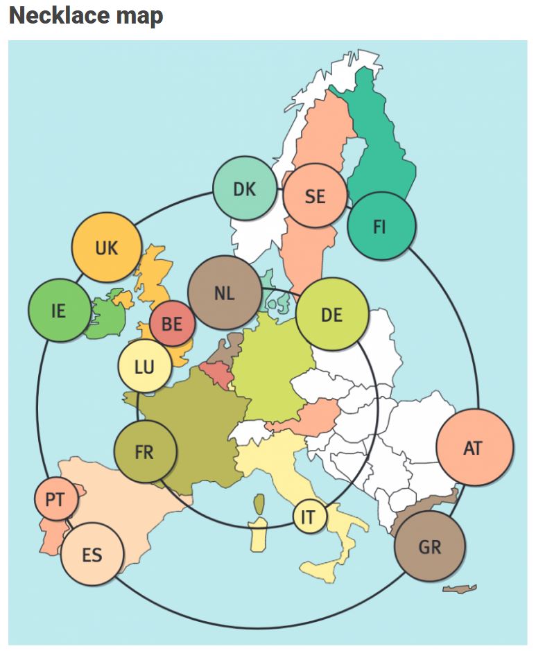
The below necklace map is new to me too. What it does precisely is unclear to me as well.

temp — In a necklace map, the regions of the underlying two-dimensional map are projected onto intervals on a one-dimensional curve (the necklace) that surrounds the map regions. Symbols are scaled such that their area corresponds to the data of their region and placed without overlap inside the corresponding interval on the necklace. [https://xeno.graphics/necklace-map/]

There are hundreds of other interestingcharts, maps, figures, and plots, so do have a look yourself. Moreover, the xenographics collection is still growing. If you know of one that isn’t here already, please submit it. You can also expect some posts about certain topics around xenographics.

ggstatsplot: Creating graphics including statistical details

This pearl had been resting in my inbox for quite a while before I was able to add it to my R resources list. Citing its GitHub page, ggstatsplot is an extension of ggplot2 package for creating graphics with details from statistical tests included in the plots themselves and targeted primarily at behavioral sciences community to provide a one-line code to produce information-rich plots. The package is currently maintained and still under development by Indrajeet Patil. Nevertheless, its functionality is already quite impressive. You can download the latest stable version via:

utils::install.packages(pkgs = "ggstatsplot")

Or download the development version via:

devtools::install_github(
  repo = "IndrajeetPatil/ggstatsplot", # package path on GitHub
  dependencies = TRUE,                 # installs packages which ggstatsplot depends on
  upgrade_dependencies = TRUE          # updates any out of date dependencies
)

The package currently supports many different statistical plots, including:

?ggbetweenstats
?ggscatterstats
?gghistostats
?ggpiestats
?ggcorrmat
?ggcoefstats
?combine_plots
?grouped_ggbetweenstats
?grouped_ggscatterstats
?grouped_gghistostats
?grouped_ggpiestats
?grouped_ggcorrmat

Let’s take a closer look at the first one:

ggbetweenstats

This function creates either a violin plot, a box plot, or a mix of two for between-group or between-condition comparisons and additional detailed results from statistical tests can be added in the subtitle. The simplest function call looks like the below, but much more complex information can be added and specified.

set.seed(123) # to get reproducible results

# the functions work approximately the same as ggplot2
ggstatsplot::ggbetweenstats(
  data = datasets::iris, 
  x = Species, 
  y = Sepal.Length,
  messages = FALSE
) +   
# and can be adjusted using the same, orginal function calls
  ggplot2::coord_cartesian(ylim = c(3, 8)) + 
  ggplot2::scale_y_continuous(breaks = seq(3, 8, by = 1))

All pictures copied from the GitHub page of ggstatsplot [original]

ggscatterstats

Not all plots are ggplot2-compatible though, for instance, ggscatterstats is not. Nevertheless, it produces a very powerful plot in my opinion.

ggstatsplot::ggscatterstats(
  data = datasets::iris, 
  x = Sepal.Length, 
  y = Petal.Length,
  title = "Dataset: Iris flower data set",
  messages = FALSE
)

ggcormat

ggcorrmat is also quite impressive, producing correlalograms with only minimal amounts of code as it wraps around ggcorplot. The defaults already produces publication-ready correlation matrices:

ggstatsplot::ggcorrmat(
  data = datasets::iris,
  corr.method = "spearman",
  sig.level = 0.005,
  cor.vars = Sepal.Length:Petal.Width,
  cor.vars.names = c("Sepal Length", "Sepal Width", "Petal Length", "Petal Width"),
  title = "Correlalogram for length measures for Iris species",
  subtitle = "Iris dataset by Anderson",
  caption = expression(
    paste(
      italic("Note"),
      ": X denotes correlation non-significant at ",
      italic("p "),
      "< 0.005; adjusted alpha"
    )
  )
)

ggcoefstats

Finally, ggcoefstats is a wrapper around GGally::ggcoef, creating a plot with the regression coefficients’ point estimates as dots with confidence interval whiskers. Here’s an example with some detailed specifications:

ggstatsplot::ggcoefstats(
  x = stats::lm(formula = mpg ~ am * cyl,
                data = datasets::mtcars),
  point.color = "red",
  vline.color = "#CC79A7",
  vline.linetype = "dotdash",
  stats.label.size = 3.5,
  stats.label.color = c("#0072B2", "#D55E00", "darkgreen"),
  title = "Car performance predicted by transmission and cylinder count",
  subtitle = "Source: 1974 Motor Trend US magazine"
) +                                    
  ggplot2::scale_y_discrete(labels = c("transmission", "cylinders", "interaction")) +
  ggplot2::labs(x = "regression coefficient",
                y = NULL)

I for one am very curious to see how Indrajeet will further develop this package, and whether academics will start using it as a default in publishing.

Generating Book Covers By Their Words — My Dissertation Cover

As some of you might know, I am defending my PhD dissertation later this year. It’s titled “Data-Driven Human Resource Management: The rise of people analytics and its application to expatriate management” and, over the past few months, I was tasked with designing its cover.

Now, I didn’t want to buy some random stock photo depicting data, an organization, or overly happy employees. I’d rather build something myself. Something reflecting what I liked about the dissertation project: statistical programming and sharing and creating knowledge with others.

Hence, I came up with the idea to use the collective intelligence of the People Analytics community to generate a unique cover. It required a dataset of people analytics-related concepts, which I asked People Analytics professionals on LinkedIn, Twitter, and other channels to help compile. Via a Google Form, colleagues, connections, acquitances, and complete strangers contributed hundreds of keywords ranging from the standard (employees, HRM, performance) to the surprising (monetization, quantitative scissors [which I had to Google]). After reviewing the list and adding some concepts of my own creation, I ended up with 1786 unique words related to either business, HRM, expatriation, data science, or statistics.

I very much dislike wordclouds (these are kind of cool though), but already had a different idea in mind. I thought of generating a background cover of the words relating to my dissertation topic, over which I could then place my title and other information. I wanted to place these keywords randomly, maybe using a color schema, or with some random sizes.

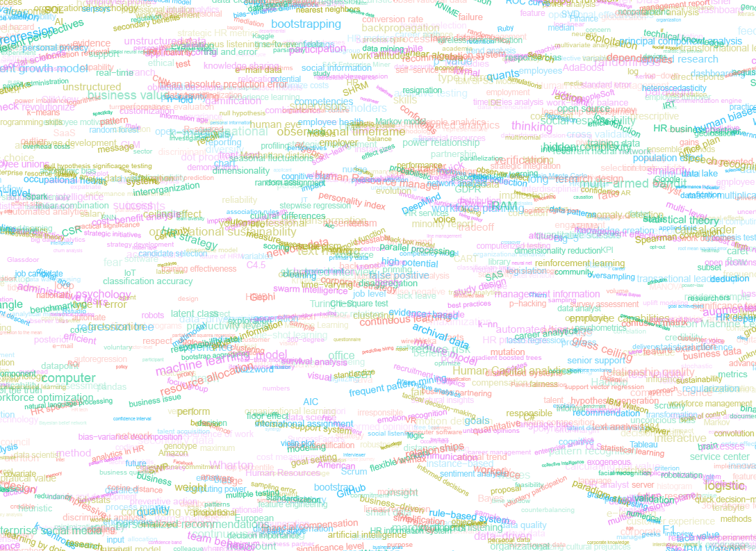
The picture below shows the result of one of my first attempts. I programmed everything in R, writing some custom functionality to generate the word-datasets, the cover-plot, and .png, .pdf, and .gif files as output.

Random colors did not produce a pleasing result and I definitely needed more and larger words in order to fill my 17cm by 24cm canvas!

Hence, I started experimenting. Using base R’s expand.grid() and set.seed() together with mapply(), I could quickly explore and generate a large amount of covers based on different parameter settings and random fluctuations.

expand.grid(seed = c(1:3), 
            dupl = c(1:4, seq(5, 30, 5)),
            font = c("sans", "League Spartan"),
            colors = c(blue_scheme, red_scheme, 
                       rainbow_scheme, random_scheme),
            size_mult = seq(1, 3, 0.3),
            angle_sd = c(5, 10, 12, 15)) -> 
  param

mapply(create_textcover, 
       param$seed, param$dupl, 
       param$font, param$colors, 
       param$size_mult, param$angle_sd)

The generation process for each unique cover only took a few seconds, so I would generate a few hundred, quickly browse through them, update the parameters to match my preferences, and then generate a new set. Among others, I varied the color palette used, the size range of the words, their angle, the font used, et cetera. To fill up the canvas, I experimented with repeating the words: two, three, five, heck, even twenty, thirty times. After an evening of generating and rating, I came to the final settings for my cover:

Words were repeated twenty times in the dataset.
Words were randomly distributed across the canvas.
Words placed in random order onto the canvas, except for a select set of relevant words, placed last.
Words’ transparency ranged randomly between 0% and 70%.
Words’ color was randomly selected out of six colors from this palette of blues.
Words’ writing angles were normally distributed around 0 degrees, with a standard deviation of 12 degrees. However, 25% of words were explicitly without angle.
Words’ size ranged between 1 and 4 based on a negative binomial distribution (10 * 0.8) resulting in more small than large words. The set of relevant words were explicitly enlarged throughout.

With League Spartan (#thisisparta) loaded as a beautiful custom font, this was the final cover background which I and my significant other liked most:

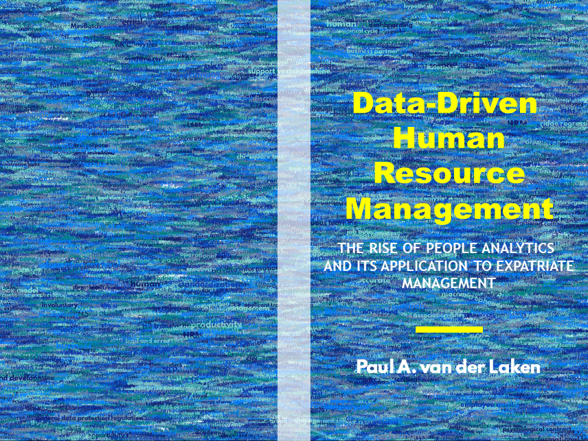
While I still need to decide on the final details regarding title placement and other details, I suspect that the final cover will look something like below — the white stripe in the middle depicting the book’s back.

Now, for the finale, I wanted to visualize the generation process via a GIF. Thomas Lin Pedersen developed this great gganimate package, which builds on the older animation package. The package greatly simplifies creating your own GIFs, as I already discussed in this earlier blog about animated GIFs in R. Anywhere, here is the generation process, where each frame includes the first frame ^ 3.2 words:

If you are interested in the process, or the R code I’ve written, feel free to reach out!

I’m sharing a digital version of the dissertation online sometime around the defense date: November 9th, 2018. If you’d like a copy, you can still leave your e-mailadress in the Google Form here and I’ll make sure you’ll receive your copy in time!