Caselaw Access Project: Structured data of over 6 million U.S. court decisions

Case.law seems like a very interesting data source for a machine learning or text mining project:

The Caselaw Access Project (“CAP”) expands public access to U.S. law. Our goal is to make all published U.S. court decisions freely available to the public online, in a consistent format, digitized from the collection of the Harvard Law Library.
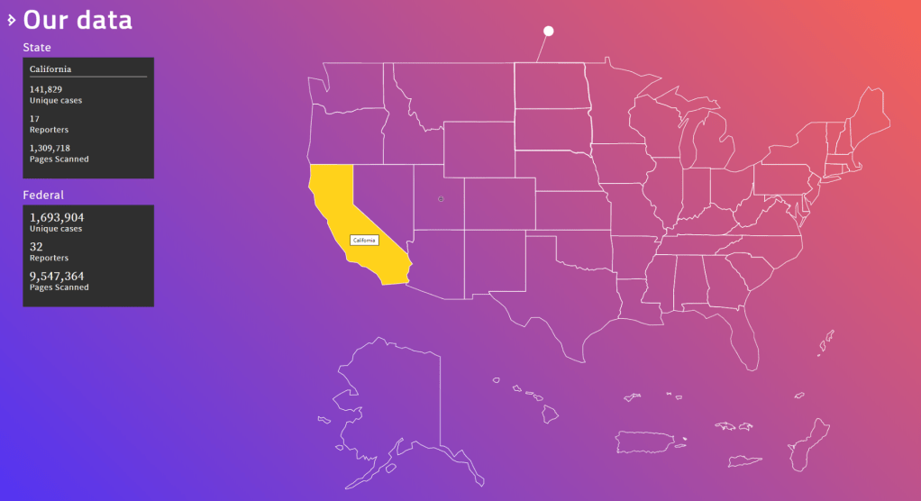
The capstone of the Caselaw Access Project is a robust set of tools which facilitate access to the cases and their associated metadata. We currently offer five ways to access the data: API, bulk downloads, search, browse, and a historical trends viewer.
https://case.law/about/

Our open-source API is the best option for anybody interested in programmatically accessing our metadata, full-text search, or individual cases.
If you need a large collection of cases, you will probably be best served by our bulk data downloads. Bulk downloads for Illinois and Arkansas are available without a login, and unlimited bulk files are available to research scholars.
https://case.law/about/

Case metadata, such as the case name, citation, court, date, etc., is freely and openly accessible without limitation. Full case text can be freely viewed or downloaded but you must register for an account to do so, and currently you may view or download no more than 500 cases per day. In addition, research scholars can qualify for bulk data access by agreeing to certain use and redistribution restrictions. You can request a bulk access agreement by creating an account and then visiting your account page.
Access limitations on full text and bulk data are a component of Harvard’s collaboration agreement with Ravel Law, Inc. (now part of Lexis-Nexis). These limitations will end, at the latest, in March of 2024. In addition, these limitations apply only to cases from jurisdictions that continue to publish their official case law in print form. Once a jurisdiction transitions from print-first publishing to digital-first publishing, these limitations cease. Thus far, Illinois and Arkansas have made this important and positive shift and, as a result, all historical cases from these jurisdictions are freely available to the public without restriction. We hope many other jurisdictions will follow their example soon.
https://case.law/about/

A different project altogether is helping the team behind Caselaw improve its data quality:

Our data inevitably includes countless errors as part of the digitization process. The public launch of this project is only the start of discovering errors, and we hope you will help us in finding and fixing them.
Some parts of our data are higher quality than others. Case metadata, such as the party names, docket number, citation, and date, has received human review. Case text and general head matter has been generated by machine OCR and has not received human review.
You can report errors of all kinds at our Github issue tracker, where you can also see currently known issues. We particularly welcome metadata corrections, feature requests, and suggestions for large-scale algorithmic changes. We are not currently able to process individual OCR corrections, but welcome general suggestions on the OCR correction process.
https://case.law/about/

OriginLab’s Graph Gallery: A blast from the past

Continuing my recent line of posts on data visualization resources, I found another repository in my inbox: OriginLab’s GraphGallery!

If I’m being honest, I would personally advice you to look at the dataviz project instead, if you haven’t heard of that one yet.

However, OriginLab might win in terms of sentiment. It has this nostalgic look of the ’90s, and apparently people really used it during that time. Nevertheless, despite looking old, the repo seems to be quite extensive, with nearly 400 different types of data visualizations:

Quantity isn’t everything though, as some of the 400 entries are disgustingly horrible:

What I do like about this OriginLab repo is that it has an option to sort its contents using a random order. This really facilitates discovery of new pearls:

Thanks to Maarten Lambrechts for sharing this resource on twitter a while back!

This visualisation tool I've never heard of is used by "500.000 scientists and engineers" and has an amazing gallery of 388 different chart types and variations https://t.co/0N3Td6jhql pic.twitter.com/A7g4DeEGEv
— Maarten Lambrechts (@maartenzam) September 20, 2019

How Booking.com deals with Selection Bias

I came across this PyData 2018 talk by Lucas Bernadi of Booking.com where he talks about the importance of selection bias for practical applications of machine learning.

We can’t just throw data into machines and expect to see any meaning […], we need to think [about this]. I see a strong trend in the practitioners community to just automate everything, to just throw data into a black box and expect to get money out of it, and I really don’t believe in that.
Lucas Bernadi in https://www.youtube.com/watch?v=3ZWCKr0vDtc

All pictures below are slides from the above video.

My summary / interpretation

Lucas highlights an example he has been working on at Booking.com, where they seek to predict which searching activities on their website are for family trips.

What happens is that people forget to specify that they intend to travel as a family, forget to input one/two/three child travellers will come along on the trip, and end up not being able to book the accomodations that come up during their search. If Booking.com would know, in advance, that people (may) be searching for family accomodations, they can better guide these bookers to family arrangements.

The problem here is that many business processes in real life look and act like a funnel. Samples drop out of the process during the course of it. So too the user search activity on Booking.com’s website acts like a funnel.

People come to search for arrangements
Less people end up actually booking arrangements
Even less people actually go on their trip
And even less people then write up a review

However, only for those people that end up writing a review, Booking.com knows 100% certain that they it concerned a family trip, as that is the moment the user can specify so. Of all other people, who did not reach stage 4 of the funnel, Booking.com has no (or not as accurate an) idea whether they were looking for family trips.

Such a funnel thus inherently produces business data with selection bias in it. Only for people making it to the review stage we know whether they were family trips or not. And only those labeled data can be used to train our machine learning model.

And now for the issue: if you train and evaluate a machine learning model on data generated with such a selection bias, your observed performance metrics will not reflect the actual performance of your machine learning model!

Actually, they are pretty much overestimates.

This is very much an issue, even though many ML practitioners don’t see aware. Selection bias makes us blind as to the real performance of our machine learning models. It produces high variance in the region of our feature space where labels are missing. This leads us to being overconfident in our ability to predict whether some user is looking for a family trip. And if the mechanism causing the selection bias is still there, we could never find out that we are overconfident. Consistently estimating, say, 30% of people are looking for family trips, whereas only 25% are.

Fortunately, Lucas proposes a very simple solution! Just adding more observations can (partially) alleviate this detrimental effect of selection bias. Although our bias still remains, the variance goes down and the difference between our observed and actual performance decreases.

A second issue and solution to selection bias relates to propensity (see also): the extent to which your features X influence not only the outcome Y, but also the selection criteria s.

If our features X influence both the outcome Y but also the selection criteria s, selection bias will occur in your data and can thus screw up your conclusion. In order to inspect to what extent this occurs in your setting, you will want to estimate a propensity model. If that model is good, and X appears valuable in predicting s, you have a selection bias problem.

Via a propensity model s ~ X, we quantify to what extent selection bias influences our data and model. The nice thing is that we, as data scientists, control the features X we use to train a model. Hence, we could just use only features X that do not predict s to predict Y. Conclusion: we can conduct propensity-based feature selection in our Y ~ X by simply avoiding features X that predicted s!

Still, Lucas does point that this becomes difficult when you have valuable features that predict both s and Y. Hence, propensity-based feature selection may end up cost(ing) you performance, as you will need to remove features relevant to Y.

I am sure I explained this phenomena worse than Lucas did himself, so please do have a look at the original PyData 2018 Amsterdam video!

Visualizing Sampling Distributions in ggplot2: Adding area under the curve

Thank you ggplot2tutor for solving one of my struggles. Apparently this is all it takes:

ggplot(NULL, aes(x = c(-3, 3))) +
  stat_function(fun = dnorm, geom = "line")

I can’t begin to count how often I have wanted to visualize a (normal) distribution in a plot. For instance to show how my sample differs from expectations, or to highlight the skewness of the scores on a particular variable. I wish I’d known earlier that I could just add one simple geom to my ggplot!

Want a different mean and standard deviation, just add a list to the args argument:

ggplot(NULL, aes(x = c(0, 20))) +
  stat_function(fun = dnorm,
                geom = "area",
                args = list(
                  mean = 10,
                  sd = 3
                ))

Need a different distribution? Just pass a different distribution function to stat_function. For instance, an F-distribution, with the df function:

ggplot(NULL, aes(x = c(0, 5))) +
  stat_function(fun = df,
                geom = "area",
                args = list(
                  df1 = 2,
                  df2 = 10
                ))

You can make it is complex as you want. The original ggplot2tutor blog provides this example:

ggplot(NULL, aes(x = c(-3, 5))) +
  stat_function(
    fun = dnorm,
    geom = "area",
    fill = "steelblue",
    alpha = .3
  ) +
  stat_function(
    fun = dnorm,
    geom = "area",
    fill = "steelblue",
    xlim = c(qnorm(.95), 4)
  ) +
  stat_function(
    fun = dnorm,
    geom = "line",
    linetype = 2,
    fill = "steelblue",
    alpha = .5,
    args = list(
      mean = 2
    )
  ) +
  labs(
    title = "Type I Error",
    x = "z-score",
    y = "Density"
  ) +
  scale_x_continuous(limits = c(-3, 5))

Have a look at the original blog here: https://ggplot2tutor.com/sampling_distribution/sampling_distribution/

Finland’s free online AI crash course

Finland developed a crash course on AI to educate its citizens. The course was arguably a great local success, with over 50 thousand Fins taking the course (1% of the population).

Now, as a gift to the European Union, Finland has opened up the course for the rest of Europe and the world to enjoy.

All pictures are screenshots taken from the website

The course is even being translated into several local languages. At the time of writing, five Northern European languages are already supported, but additional translation efforts are still in progress.

Elements of AI takes six weeks and functions as a crash course and beginner introduction to the field of AI:

treevis.net – A Visual Bibliography of Tree Visualizations

Last week I cohosted a professional learning course on data visualization at JADS. My fellow host was prof. Jack van Wijk, and together we organized an amazing workshop and poster event. Jack gave two lectures on data visualization theory and resources, and mentioned among others treevis.net, a resource I was unfamiliar with up until then.

treevis.net is a lot like the dataviz project in the sense that it is an extensive overview of different types of data visualizations. treevis is unique, however, in the sense that it is focused on specifically visualizations of hierarchical data: multi-level or nested data structures.

Hans-Jörg Schulz — professor of Computer Science at Aarhus University in Denmark — maintains the treevis repo. At the moment of writing, he has compiled over 300 different types of hierachical data visualizations and displays them on this website.

As an added bonus, the repo is interactive as there are several ways to filter and look for the visualization type that best fits your data and needs.

Most resources come with added links to the original authors and the original papers they were first published in, so this is truly a great resources for those interested in doing a deep dive into data visualization. Do have a look yourself!