Continuing my recent line of posts on data visualization resources, I found another repository in my inbox: OriginLab’s GraphGallery!
If I’m being honest, I would personally advice you to look at the dataviz project instead, if you haven’t heard of that one yet.
However, OriginLab might win in terms of sentiment. It has this nostalgic look of the ’90s, and apparently people really used it during that time. Nevertheless, despite looking old, the repo seems to be quite extensive, with nearly 400 different types of data visualizations:
Quantity isn’t everything though, as some of the 400 entries are disgustingly horrible:
There’s so much wrong with this graph…
What I do like about this OriginLab repo is that it has an option to sort its contents using a random order. This really facilitates discovery of new pearls:
Thanks to Maarten Lambrechts for sharing this resource on twitter a while back!
This visualisation tool I've never heard of is used by "500.000 scientists and engineers" and has an amazing gallery of 388 different chart types and variations https://t.co/0N3Td6jhqlpic.twitter.com/A7g4DeEGEv
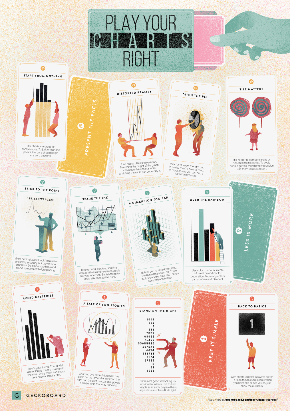
In a world where data really matters, we all want to create effective charts. But data visualization is rarely taught in schools, or covered in on-the-job training. Most of us learn as we go along, and therefore we often make choices or mistakes that confuse and disorient our audience. From overcomplicating or overdressing our charts, to conveying an entirely inaccurate message, there are common design pitfalls that can easily be avoided. We’ve put together these pointers to help you create simpler charts that effectively get across the meaning of your data.
Based on work by experts such as Stephen Few, Dona Wong, Albert Cairo, Cole Nussbaumer Knaflic, and Andy Kirk, the authors at Geckoboard wrote down a list of recommendations which I summarize below:
Present the facts
Start your axis at zero whenever possible, to prevent misinterpretation. Particularly bar charts.
The width and height of line and scatter plots influence its messages.
Area and size are hard to interpret. Hence, there’s often a better alternative to the pie chart. Read also this.
Last year witnessed the creation of many novel types of data visualization. Some lesser known ones, jokingly referred to as xenographics, I already discussed.
Two new visualization formats seem to stick around though. And as always, it was not long before someone created special R packages for them. Get ready to meet waffleplots and swarmplots!
Waffleplot
Waffleplots — also called square pie charts — are very useful in communicating parts of a whole for categorical quantities. Bob Rudis (twitter) — scholar and R developer among many other things — did us all a favor and created the R waffle package.
First, we need to install and load the waffle package.
install.packages("waffle") # install waffle package
library(waffle) # load in package
I will use the famous iris data to demonstrate both plots.
Since waffleplots work with frequencies, I will specifically use the iris$Species data stored as a frequency table.
Here, we see every single flower in the iris dataset represented by a tile. This provides an immediate visual representation of the group sizes in the dataset. Looks pretty huh!
But we can play around with the display settings, for instance, let’s change the number of rows and the placement of the legend. Building on ggplot2, the waffle package works very intuitive:
waffle(spec, rows = 3, legend_pos = "bottom")
Or, in case we want to highlight a specific value, we could play around with the colors a bit.
The plot is a bit crowded though with each flower as a seperate tile. We can simply reduce the number of tiles by dividing the values in our frequency table, like so:
# do not forget to annotate what each square represents!
w1 <- waffle(spec / 10, rows = 5, xlab = "1 square = 10 flowers")
w1
Finally, you might want to combine multiple waffles into a single visual. This you can do with the accompanied well-named waffle::iron function. Like so:
I am definately going to use this package in my daily work. I just love the visual simplicity.
As a final remark, the waffle Github page argues that the argument use_glyph can be used to replace the tiles by pictures from the extrafont package, however, I could not get the code to work.
The visual resulting from the use_glyph waffle example via github.
The ggplot2 waffle extension geom_waffle is being developed as we speak, but is not yet hosted on CRAN yet.
Some examples hosted on the Github page also use the iris dataset, so you can have a look at those. However, I made novel visuals because I prefer theme_light. Hence, I first install the ggbeeswarm package along with ggplot2, and then set the default theme to theme_light.
As this is an “official” ggplot2 extension, most functionality works the same as in any other geom_*. Thus, adding colors or increasing point size is easy:
ggplot(iris, aes(Species, Sepal.Length, col = Species)) + geom_beeswarm(size = 2)
For larger sizes, you might want to adjust the spacing between the points using the cex argument.
Points in a beeswarmplot are automatically plotted side-by-side grouped on the X variable, but you can turn that off with the groupOnX command.
ggplot(iris, aes(Species, Sepal.Length, col = Species)) + geom_beeswarm(groupOnX = FALSE)
Finally, if you have another grouping variable besides those on the axis (e.g., a large Sepal.Length below), you might want to consider using the dodge.width argument to seperate the groups.
The second function in the ggbeeswarm package is geom_quasirandom, an alternative to the original geom_jitter. Basically, it’s a convenient tool to offset points within categories to reduce overplotting.
ggplot(iris, aes(Species, Sepal.Length, col = Species)) + geom_quasirandom()
Instead of the quasirandom offset, the geom allows for many other methods, including a smiley face pattern : )
There is also a earlier package on CRAN, called beeswarm, but it doesn’t seem to be maintained anymore. Moreover, its syntax more or less resembles R’s base::plot, whereas I have a strong preference for ggplot2 personally.
I’ve mentioned before that I dislike wordclouds (for instance here, or here) and apparently others share that sentiment. In his recent Medium blog, Daniel McNichol goes as far as to refer to the wordcloud as the pie chart of text data! Among others, Daniel calls wordclouds disorienting, one-dimensional, arbitrary and opaque and he mentions their lack of order, information, and scale.
Wordcloud of the negative characteristics of wordclouds, via Medium
Instead of using wordclouds, Daniel suggests we revert to alternative approaches. For instance, in their Tidy Text Mining with R book, Julia Silge and David Robinson suggest using bar charts or network graphs, providing the necessary R code. Another alternative is provided in Daniel’s blog: the chatterplot!
While Daniel didn’t invent this unorthodox wordcloud-like plot, he might have been the first to name it a chatterplot. Daniel’s chatterplot uses a full x/y cartesian plane, turning the usually only arbitrary though exploratory wordcloud into a more quantitatively sound, information-rich visualization.
R package ggplot’s geom_text() function — or alternatively ggrepel‘s geom_text_repel() for better legibility — is perfectly suited for making a chatterplot. And interesting features/variables for the axis — apart from the regular word frequencies — can be easily computed using the R tidytext package.
Here’s an example generated by Daniel, plotting words simulatenously by their frequency of occurance in comments to Hacker News articles (y-axis) as well as by the respective popularity of the comments the word was used in (log of the ranking, on the x-axis).
[CHATTERPLOTs are] like a wordcloud, except there’s actual quantitative logic to the order, placement & aesthetic aspects of the elements, along with an explicit scale reference for each. This allows us to represent more, multidimensional information in the plot, & provides the viewer with a coherent visual logic& direction by which to explore the data.
I highly recommend the use of these chatterplots over their less-informative wordcloud counterpart, and strongly suggest you read Daniel’s original blog, in which you can also find the R code for the above visualizations.
A recent open access paper by Nicholas Tierney and Dianne Cook — professors at Monash University — deals with simpler handling, exploring, and imputation of missing values in data.They present new methodology building upon tidy data principles, with a goal to integrating missing value handling as an integral part of data analysis workflows. New data structures are defined (like the nabular) along with new functions to perform common operations (like gg_miss_case).
These new methods have bundled among others in the R packages naniar and visdat, which I highly recommend you check out. To put in the author’s own words:
The naniar and visdat packages build on existing tidy tools and strike a compromise between automation and control that makes analysis efficient, readable, but not overly complex. Each tool has clear intent and effects – plotting or generating data or augmenting data in some way. This reduces repetition and typing for the user, making exploration of missing values easier as they follow consistent rules with a declarative interface.
The below showcases some of the highly informational visuals you can easily generate with naniar‘s nabulars and the associated functionalities.
For instance, these heatmap visualizations of missing data for the airquality dataset. (A) represents the default output and (B) is ordered by clustering on rows and columns. You can see there are only missings in ozone and solar radiation, and there appears to be some structure to their missingness.
Another example is this upset plot of the patterns of missingness in the airquality dataset. Only Ozone and Solar.R have missing values, and Ozone has the most missing values. There are 2 cases where both Solar.R and Ozone have missing values.
You can also generate a histogram using nabular data in order to show the values and missings in Ozone. Values are imputed below the range to show the number of missings in Ozone and colored according to missingness of ozone (‘Ozone_NA‘). This displays directly that there are approximately 35-40 missings in Ozone.
Alternatively, scatterplots can be easily generated. Displaying missings at 10 percent below the minimum of the airquality dataset. Scatterplots of ozone and solar radiation (A), and ozone and temperature (B). These plots demonstrate that there are missings in ozone and solar radiation, but not in temperature.
Finally, this parallel coordinate plot displays the missing values imputed 10% below range for the oceanbuoys dataset. Values are colored by missingness of humidity. Humidity is missing for low air and sea temperatures, and is missing for one year and one location.
Laura DeCicco found that non-R users keep asking her what her box plots exactly mean or demonstrate. In a recent blog post, she therefore breaks down the calculations into easy-to-follow chunks of code. Even better, she included the source code to make boxplots that come with a very elaborate default legend:
As you can see, the above contains much more and easier to understand information than the original ggplot2 boxplot below.
Laura wrote the custom function ggplot_box_legend() (see source code below and in Laura’s blog), which uses the cowplot package to paste the explanation to the box plot. All you need to do is call the legend function just before you run your ggplot2 boxplot call.
ggplot_box_legend <- function(family = "serif"){

  # Create data to use in the boxplot legend:
  set.seed(100)

  sample_df <- data.frame(parameter = "test",
                        values = sample(500))

  # Extend the top whisker a bit:
  sample_df$values[1:100] <- 701:800
  # Make sure there's only 1 lower outlier:
  sample_df$values[1] <- -350

  # Function to calculate important values:
  ggplot2_boxplot <- function(x){

    quartiles <- as.numeric(quantile(x,
                                     probs = c(0.25, 0.5, 0.75)))

    names(quartiles) <- c("25th percentile",
                          "50th percentile\n(median)",
                          "75th percentile")

    IQR <- diff(quartiles[c(1,3)])

    upper_whisker <- max(x[x < (quartiles[3] + 1.5 * IQR)])
    lower_whisker <- min(x[x > (quartiles[1] - 1.5 * IQR)])

    upper_dots <- x[x > (quartiles[3] + 1.5*IQR)]
    lower_dots <- x[x < (quartiles[1] - 1.5*IQR)]

    return(list("quartiles" = quartiles,
                "25th percentile" = as.numeric(quartiles[1]),
                "50th percentile\n(median)" = as.numeric(quartiles[2]),
                "75th percentile" = as.numeric(quartiles[3]),
                "IQR" = IQR,
                "upper_whisker" = upper_whisker,
                "lower_whisker" = lower_whisker,
                "upper_dots" = upper_dots,
                "lower_dots" = lower_dots))
  }

  # Get those values:
  ggplot_output <- ggplot2_boxplot(sample_df$values)

  # Lots of text in the legend, make it smaller and consistent font:
  update_geom_defaults("text",
                     list(size = 3,
                          hjust = 0,
                          family = family))
  # Labels don't inherit text:
  update_geom_defaults("label",
                     list(size = 3,
                          hjust = 0,
                          family = family))

  # Create the legend:
  # The main elements of the plot (the boxplot, error bars, and count)
  # are the easy part.
  # The text describing each of those takes a lot of fiddling to
  # get the location and style just right:
  explain_plot <- ggplot() +     stat_boxplot(data = sample_df,                  aes(x = parameter, y=values),                  geom ='errorbar', width = 0.3) +     geom_boxplot(data = sample_df,                  aes(x = parameter, y=values),                   width = 0.3, fill = "lightgrey") +     geom_text(aes(x = 1, y = 950, label = "500"), hjust = 0.5) +     geom_text(aes(x = 1.17, y = 950,                   label = "Number of values"),               fontface = "bold", vjust = 0.4) +     theme_minimal(base_size = 5, base_family = family) +     geom_segment(aes(x = 2.3, xend = 2.3,                       y = ggplot_output[["25th percentile"]],                       yend = ggplot_output[["75th percentile"]])) +     geom_segment(aes(x = 1.2, xend = 2.3,                       y = ggplot_output[["25th percentile"]],                       yend = ggplot_output[["25th percentile"]])) +     geom_segment(aes(x = 1.2, xend = 2.3,                       y = ggplot_output[["75th percentile"]],                       yend = ggplot_output[["75th percentile"]])) +     geom_text(aes(x = 2.4, y = ggplot_output[["50th percentile\n(median)"]]),                label = "Interquartile\nrange", fontface = "bold",               vjust = 0.4) +     geom_text(aes(x = c(1.17,1.17),                    y = c(ggplot_output[["upper_whisker"]],                         ggplot_output[["lower_whisker"]]),                    label = c("Largest value within 1.5 times\ninterquartile range above\n75th percentile",                             "Smallest value within 1.5 times\ninterquartile range below\n25th percentile")),                   fontface = "bold", vjust = 0.9) +     geom_text(aes(x = c(1.17),                    y =  ggplot_output[["lower_dots"]],                    label = "Outside value"),                vjust = 0.5, fontface = "bold") +     geom_text(aes(x = c(1.9),                    y =  ggplot_output[["lower_dots"]],                    label = "-Value is >1.5 times and"),
              vjust = 0.5) +
    geom_text(aes(x = 1.17,
                  y = ggplot_output[["lower_dots"]],
                  label = "<3 times the interquartile range\nbeyond either end of the box"),
              vjust = 1.5) +
    geom_label(aes(x = 1.17, y = ggplot_output[["quartiles"]],
                  label = names(ggplot_output[["quartiles"]])),
              vjust = c(0.4,0.85,0.4),
              fill = "white", label.size = 0) +
    ylab("") + xlab("") +
    theme(axis.text = element_blank(),
          axis.ticks = element_blank(),
          panel.grid = element_blank(),
          aspect.ratio = 4/3,
          plot.title = element_text(hjust = 0.5, size = 10)) +
    coord_cartesian(xlim = c(1.4,3.1), ylim = c(-600, 900)) +
    labs(title = "EXPLANATION")

  return(explain_plot)

}

ggplot_box_legend()


 Alternatively, scatterplots can be easily generated. Displaying missings at 10 percent below the minimum of the airquality dataset. Scatterplots of ozone and solar radiation (A), and ozone and temperature (B). These plots demonstrate that there are missings in ozone and solar radiation, but not in temperature.


