Tag: visualization

Xenographics: Unusual charts and maps

Xeno.graphics is the collection of unusual charts and maps Maarten Lambrechts maintains. It’s a repository of novel, innovative, and experimental visualizations to inspire you, to fight xenographphobia, and popularize new chart types.

For instance, have you ever before heard of a time curve? These are very useful to visualize the development of a relationship over time.

Time curves are based on the metaphor of folding a timeline visualization into itself so as to bring similar time points close to each other. This metaphor can be applied to any dataset where a similarity metric between temporal snapshots can be defined, thus it is largely datatype-agnostic. [https://xeno.graphics/time-curve]

The upset plot is another example of an upcoming visualization. It can demonstrate the overlap or insection in a dataset. For instance, in the social network of #rstats twitter heroes, as the below example from the Xenographics website does.

Understanding relationships between sets is an important analysis task. The major challenge in this context is the combinatorial explosion of the number of set intersections if the number of sets exceeds a trivial threshold. To address this, we introduce UpSet, a novel visualization technique for the quantitative analysis of sets, their intersections, and aggregates of intersections. [https://xeno.graphics/upset-plot/]

The below necklace map is new to me too. What it does precisely is unclear to me as well.

temp — In a necklace map, the regions of the underlying two-dimensional map are projected onto intervals on a one-dimensional curve (the necklace) that surrounds the map regions. Symbols are scaled such that their area corresponds to the data of their region and placed without overlap inside the corresponding interval on the necklace. [https://xeno.graphics/necklace-map/]

There are hundreds of other interestingcharts, maps, figures, and plots, so do have a look yourself. Moreover, the xenographics collection is still growing. If you know of one that isn’t here already, please submit it. You can also expect some posts about certain topics around xenographics.

ggstatsplot: Creating graphics including statistical details

This pearl had been resting in my inbox for quite a while before I was able to add it to my R resources list. Citing its GitHub page, ggstatsplot is an extension of ggplot2 package for creating graphics with details from statistical tests included in the plots themselves and targeted primarily at behavioral sciences community to provide a one-line code to produce information-rich plots. The package is currently maintained and still under development by Indrajeet Patil. Nevertheless, its functionality is already quite impressive. You can download the latest stable version via:

utils::install.packages(pkgs = "ggstatsplot")

Or download the development version via:

devtools::install_github(
  repo = "IndrajeetPatil/ggstatsplot", # package path on GitHub
  dependencies = TRUE,                 # installs packages which ggstatsplot depends on
  upgrade_dependencies = TRUE          # updates any out of date dependencies
)

The package currently supports many different statistical plots, including:

?ggbetweenstats
?ggscatterstats
?gghistostats
?ggpiestats
?ggcorrmat
?ggcoefstats
?combine_plots
?grouped_ggbetweenstats
?grouped_ggscatterstats
?grouped_gghistostats
?grouped_ggpiestats
?grouped_ggcorrmat

Let’s take a closer look at the first one:

ggbetweenstats

This function creates either a violin plot, a box plot, or a mix of two for between-group or between-condition comparisons and additional detailed results from statistical tests can be added in the subtitle. The simplest function call looks like the below, but much more complex information can be added and specified.

set.seed(123) # to get reproducible results

# the functions work approximately the same as ggplot2
ggstatsplot::ggbetweenstats(
  data = datasets::iris, 
  x = Species, 
  y = Sepal.Length,
  messages = FALSE
) +   
# and can be adjusted using the same, orginal function calls
  ggplot2::coord_cartesian(ylim = c(3, 8)) + 
  ggplot2::scale_y_continuous(breaks = seq(3, 8, by = 1))

All pictures copied from the GitHub page of ggstatsplot [original]

ggscatterstats

Not all plots are ggplot2-compatible though, for instance, ggscatterstats is not. Nevertheless, it produces a very powerful plot in my opinion.

ggstatsplot::ggscatterstats(
  data = datasets::iris, 
  x = Sepal.Length, 
  y = Petal.Length,
  title = "Dataset: Iris flower data set",
  messages = FALSE
)

ggcormat

ggcorrmat is also quite impressive, producing correlalograms with only minimal amounts of code as it wraps around ggcorplot. The defaults already produces publication-ready correlation matrices:

ggstatsplot::ggcorrmat(
  data = datasets::iris,
  corr.method = "spearman",
  sig.level = 0.005,
  cor.vars = Sepal.Length:Petal.Width,
  cor.vars.names = c("Sepal Length", "Sepal Width", "Petal Length", "Petal Width"),
  title = "Correlalogram for length measures for Iris species",
  subtitle = "Iris dataset by Anderson",
  caption = expression(
    paste(
      italic("Note"),
      ": X denotes correlation non-significant at ",
      italic("p "),
      "< 0.005; adjusted alpha"
    )
  )
)

ggcoefstats

Finally, ggcoefstats is a wrapper around GGally::ggcoef, creating a plot with the regression coefficients’ point estimates as dots with confidence interval whiskers. Here’s an example with some detailed specifications:

ggstatsplot::ggcoefstats(
  x = stats::lm(formula = mpg ~ am * cyl,
                data = datasets::mtcars),
  point.color = "red",
  vline.color = "#CC79A7",
  vline.linetype = "dotdash",
  stats.label.size = 3.5,
  stats.label.color = c("#0072B2", "#D55E00", "darkgreen"),
  title = "Car performance predicted by transmission and cylinder count",
  subtitle = "Source: 1974 Motor Trend US magazine"
) +                                    
  ggplot2::scale_y_discrete(labels = c("transmission", "cylinders", "interaction")) +
  ggplot2::labs(x = "regression coefficient",
                y = NULL)

I for one am very curious to see how Indrajeet will further develop this package, and whether academics will start using it as a default in publishing.

Generating Book Covers By Their Words — My Dissertation Cover

As some of you might know, I am defending my PhD dissertation later this year. It’s titled “Data-Driven Human Resource Management: The rise of people analytics and its application to expatriate management” and, over the past few months, I was tasked with designing its cover.

Now, I didn’t want to buy some random stock photo depicting data, an organization, or overly happy employees. I’d rather build something myself. Something reflecting what I liked about the dissertation project: statistical programming and sharing and creating knowledge with others.

Hence, I came up with the idea to use the collective intelligence of the People Analytics community to generate a unique cover. It required a dataset of people analytics-related concepts, which I asked People Analytics professionals on LinkedIn, Twitter, and other channels to help compile. Via a Google Form, colleagues, connections, acquitances, and complete strangers contributed hundreds of keywords ranging from the standard (employees, HRM, performance) to the surprising (monetization, quantitative scissors [which I had to Google]). After reviewing the list and adding some concepts of my own creation, I ended up with 1786 unique words related to either business, HRM, expatriation, data science, or statistics.

I very much dislike wordclouds (these are kind of cool though), but already had a different idea in mind. I thought of generating a background cover of the words relating to my dissertation topic, over which I could then place my title and other information. I wanted to place these keywords randomly, maybe using a color schema, or with some random sizes.

The picture below shows the result of one of my first attempts. I programmed everything in R, writing some custom functionality to generate the word-datasets, the cover-plot, and .png, .pdf, and .gif files as output.

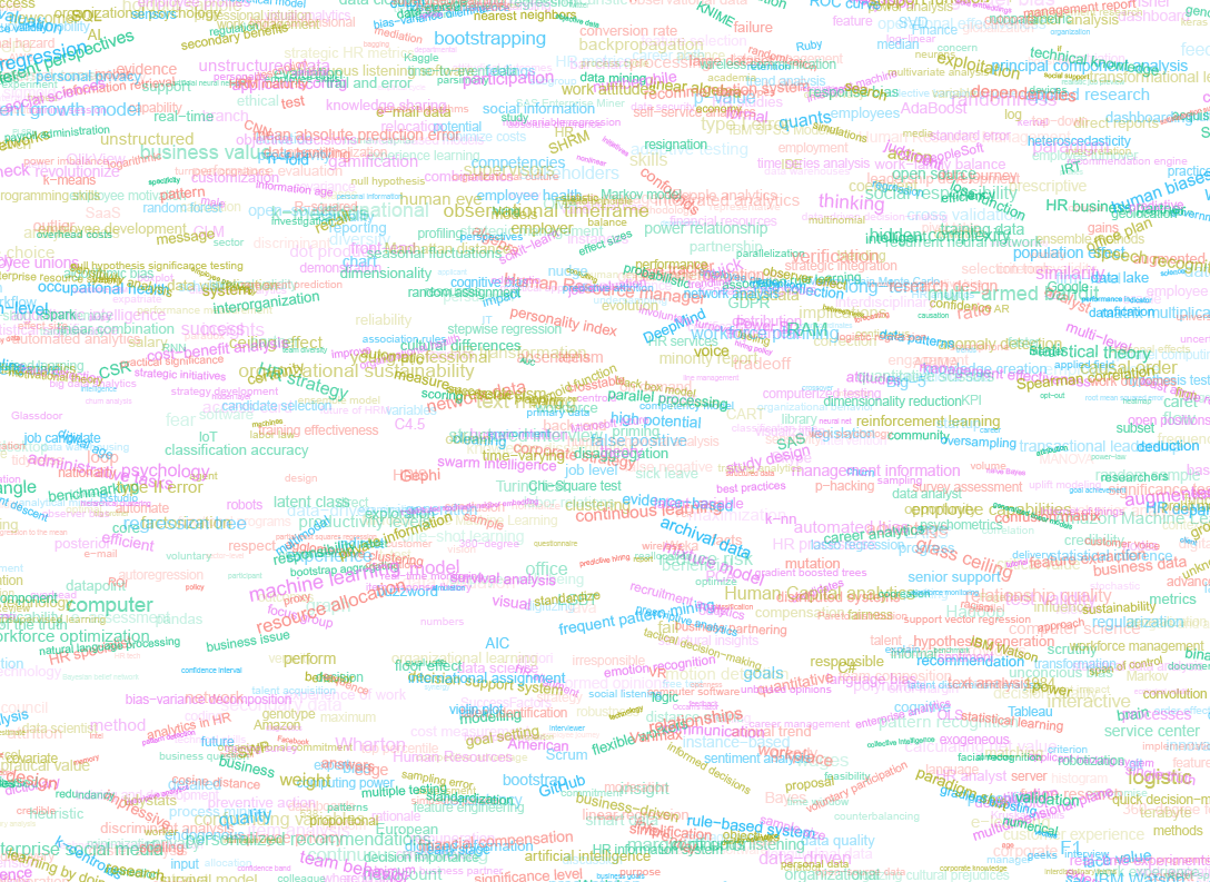
Random colors did not produce a pleasing result and I definitely needed more and larger words in order to fill my 17cm by 24cm canvas!

Hence, I started experimenting. Using base R’s expand.grid() and set.seed() together with mapply(), I could quickly explore and generate a large amount of covers based on different parameter settings and random fluctuations.

expand.grid(seed = c(1:3), 
            dupl = c(1:4, seq(5, 30, 5)),
            font = c("sans", "League Spartan"),
            colors = c(blue_scheme, red_scheme, 
                       rainbow_scheme, random_scheme),
            size_mult = seq(1, 3, 0.3),
            angle_sd = c(5, 10, 12, 15)) -> 
  param

mapply(create_textcover, 
       param$seed, param$dupl, 
       param$font, param$colors, 
       param$size_mult, param$angle_sd)

The generation process for each unique cover only took a few seconds, so I would generate a few hundred, quickly browse through them, update the parameters to match my preferences, and then generate a new set. Among others, I varied the color palette used, the size range of the words, their angle, the font used, et cetera. To fill up the canvas, I experimented with repeating the words: two, three, five, heck, even twenty, thirty times. After an evening of generating and rating, I came to the final settings for my cover:

Words were repeated twenty times in the dataset.
Words were randomly distributed across the canvas.
Words placed in random order onto the canvas, except for a select set of relevant words, placed last.
Words’ transparency ranged randomly between 0% and 70%.
Words’ color was randomly selected out of six colors from this palette of blues.
Words’ writing angles were normally distributed around 0 degrees, with a standard deviation of 12 degrees. However, 25% of words were explicitly without angle.
Words’ size ranged between 1 and 4 based on a negative binomial distribution (10 * 0.8) resulting in more small than large words. The set of relevant words were explicitly enlarged throughout.

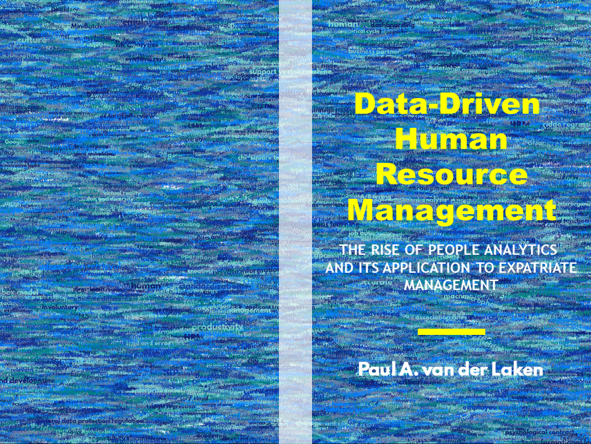
With League Spartan (#thisisparta) loaded as a beautiful custom font, this was the final cover background which I and my significant other liked most:

While I still need to decide on the final details regarding title placement and other details, I suspect that the final cover will look something like below — the white stripe in the middle depicting the book’s back.

Now, for the finale, I wanted to visualize the generation process via a GIF. Thomas Lin Pedersen developed this great gganimate package, which builds on the older animation package. The package greatly simplifies creating your own GIFs, as I already discussed in this earlier blog about animated GIFs in R. Anywhere, here is the generation process, where each frame includes the first frame ^ 3.2 words:

If you are interested in the process, or the R code I’ve written, feel free to reach out!

I’m sharing a digital version of the dissertation online sometime around the defense date: November 9th, 2018. If you’d like a copy, you can still leave your e-mailadress in the Google Form here and I’ll make sure you’ll receive your copy in time!

Multimapping in R, by Ilya Kashnitsky

Nothing beats a aesthetically-pleasing data visualization in the form of a map (see evidence here, here, here, or here).

Moreover, we’ve already witnessed some great R tutorials by Ilya Kashnitsky before (see Animated Snow in R).

These two come together in Ilya’s recent post on subplots in ggplot2 maps, with which he completely amazed me. The creation process is actually easier than the end result makes it look: make several visualizations and add them as ggplot2::annotation_custom() to your main ggplot2 map — the same as if you are adding a logo to your plot. Enjoy:

Here you can find Ilya’s original blog and the associated R script.

Interactive Explanation of Network and Graph Principles

Why do groups of people act smart, dumb, kind, or cruel? People behave in strange ways, particularly when they are able to influence one another. Both good and bad things can happen when people interact and behave in network structures. On the bright side, you must be familiar with the wisdom of the crowd, where the aggregated knowledge of a group is more valuable than its sum? Ensemble algorithms – like random forest analysis – rely on this positive principle.

On the dark side, are you familiar with the phenomenon called the tragedy of the commons, where shared resource-systems collapse because individuals behave in their self-interest? Or psychological phenomena such as groupthink, where groups of people make irrational decisions due to social issues? The recent spread of fake news and misinformation is also stimulated by network interactions. In these cases, we could speak of the madness of the crowd.

Nicky Case made a great interactive walkthrough explaining why and when networks of people become wise or mad. You are tasked to change and simulate network interactions while Nicky explains concepts such as (complex) contagion, the majority illusion paradox, bonding and bridging, and small world networks. In the references, Nicky provides links to scientific papers explaining these concepts in more detail. I highly suggest you check out her website here.

Screenshot of one of the explanations/simulations Nicky offers.

A Categorical Spatial Interpolation Tutorial in R

Timo Grossenbacher works as reporter/coder for SRF Data, the data journalism unit of Swiss Radio and TV. He analyzes and visualizes data and investigates data-driven stories. On his website, he hosts a growing list of cool projects. One of his recent blogs covers categorical spatial interpolation in R. The end result of that blog looks amazing:

This map was built with data Timo crowdsourced for one of his projects. With this data, Timo took the following steps, which are covered in his tutorial:

Read in the data, first the geometries (Germany political boundaries), then the point data upon which the interpolation will be based on.
Preprocess the data (simplify geometries, convert CSV point data into an sf object, reproject the geodata into the ETRS CRS, clip the point data to Germany, so data outside of Germany is discarded).
Then, a regular grid (a raster without “data”) is created. Each grid point in this raster will later be interpolated from the point data.
Run the spatial interpolation with the kknn package. Since this is quite computationally and memory intensive, the resulting raster is split up into 20 batches, and each batch is computed by a single CPU core in parallel.
Visualize the resulting raster with ggplot2.

All code for the above process can be accessed on Timo’s Github. The georeferenced points underlying the interpolation look like the below, where each point represents the location of a person who selected a certain pronunciation in an online survey. More details on the crowdsourced pronunciation project van be found here, .