Category: machine learning

How Booking.com deals with Selection Bias

How Booking.com deals with Selection Bias

I came across this PyData 2018 talk by Lucas Bernadi of Booking.com where he talks about the importance of selection bias for practical applications of machine learning.

We can’t just throw data into machines and expect to see any meaning […], we need to think [about this]. I see a strong trend in the practitioners community to just automate everything, to just throw data into a black box and expect to get money out of it, and I really don’t believe in that.

Lucas Bernadi in https://www.youtube.com/watch?v=3ZWCKr0vDtc

All pictures below are slides from the above video.

My summary / interpretation

Lucas highlights an example he has been working on at Booking.com, where they seek to predict which searching activities on their website are for family trips.

What happens is that people forget to specify that they intend to travel as a family, forget to input one/two/three child travellers will come along on the trip, and end up not being able to book the accomodations that come up during their search. If Booking.com would know, in advance, that people (may) be searching for family accomodations, they can better guide these bookers to family arrangements.

The problem here is that many business processes in real life look and act like a funnel. Samples drop out of the process during the course of it. So too the user search activity on Booking.com’s website acts like a funnel.

  1. People come to search for arrangements
  2. Less people end up actually booking arrangements
  3. Even less people actually go on their trip
  4. And even less people then write up a review

However, only for those people that end up writing a review, Booking.com knows 100% certain that they it concerned a family trip, as that is the moment the user can specify so. Of all other people, who did not reach stage 4 of the funnel, Booking.com has no (or not as accurate an) idea whether they were looking for family trips.

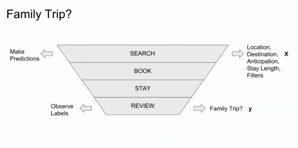
Such a funnel thus inherently produces business data with selection bias in it. Only for people making it to the review stage we know whether they were family trips or not. And only those labeled data can be used to train our machine learning model.

And now for the issue: if you train and evaluate a machine learning model on data generated with such a selection bias, your observed performance metrics will not reflect the actual performance of your machine learning model!

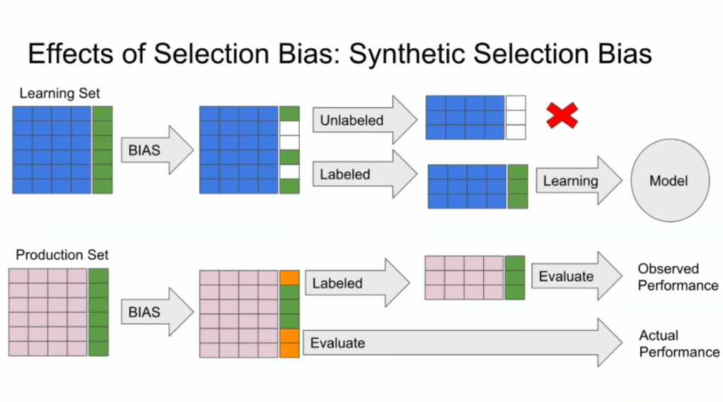
Actually, they are pretty much overestimates.

This is very much an issue, even though many ML practitioners don’t see aware. Selection bias makes us blind as to the real performance of our machine learning models. It produces high variance in the region of our feature space where labels are missing. This leads us to being overconfident in our ability to predict whether some user is looking for a family trip. And if the mechanism causing the selection bias is still there, we could never find out that we are overconfident. Consistently estimating, say, 30% of people are looking for family trips, whereas only 25% are.

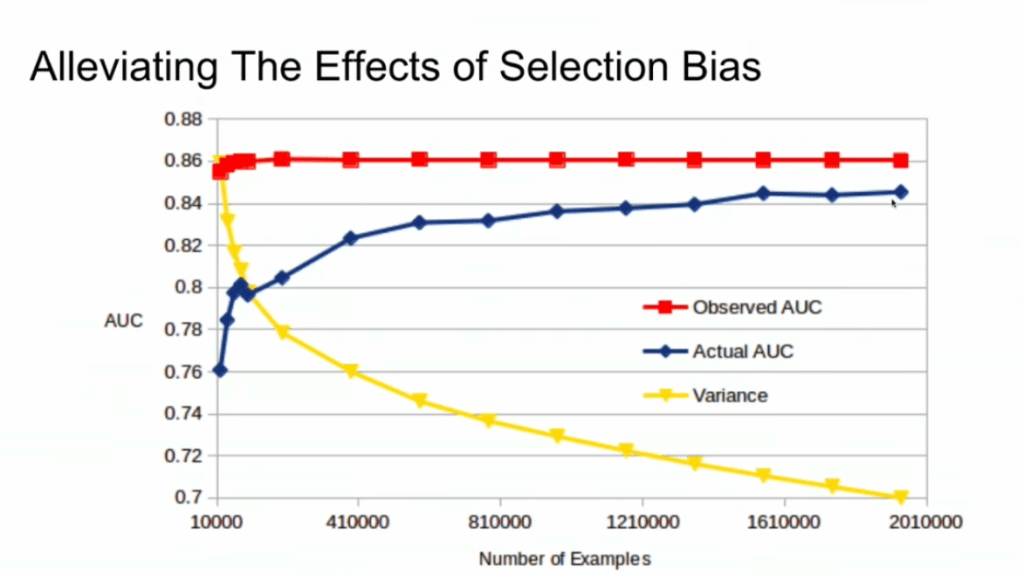
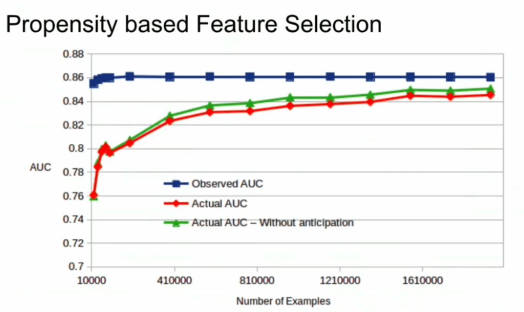
Fortunately, Lucas proposes a very simple solution! Just adding more observations can (partially) alleviate this detrimental effect of selection bias. Although our bias still remains, the variance goes down and the difference between our observed and actual performance decreases.

A second issue and solution to selection bias relates to propensity (see also): the extent to which your features X influence not only the outcome Y, but also the selection criteria s.

If our features X influence both the outcome Y but also the selection criteria s, selection bias will occur in your data and can thus screw up your conclusion. In order to inspect to what extent this occurs in your setting, you will want to estimate a propensity model. If that model is good, and X appears valuable in predicting s, you have a selection bias problem.

Via a propensity model s ~ X, we quantify to what extent selection bias influences our data and model. The nice thing is that we, as data scientists, control the features X we use to train a model. Hence, we could just use only features X that do not predict s to predict Y. Conclusion: we can conduct propensity-based feature selection in our Y ~ X by simply avoiding features X that predicted s!

Still, Lucas does point that this becomes difficult when you have valuable features that predict both s and Y. Hence, propensity-based feature selection may end up cost(ing) you performance, as you will need to remove features relevant to Y.

I am sure I explained this phenomena worse than Lucas did himself, so please do have a look at the original PyData 2018 Amsterdam video!

Finland’s free online AI crash course

Finland’s free online AI crash course

Finland developed a crash course on AI to educate its citizens. The course was arguably a great local success, with over 50 thousand Fins taking the course (1% of the population).

Now, as a gift to the European Union, Finland has opened up the course for the rest of Europe and the world to enjoy.

All pictures are screenshots taken from the website

The course is even being translated into several local languages. At the time of writing, five Northern European languages are already supported, but additional translation efforts are still in progress.

Elements of AI takes six weeks and functions as a crash course and beginner introduction to the field of AI:

Anomaly Detection Resources

Anomaly Detection Resources

Carnegie Mellon PhD student Yue Zhao collects this great Github repository of anomaly detection resources: https://github.com/yzhao062/anomaly-detection-resources

The repository consists of tools for multiple languages (R, Python, Matlab, Java) and resources in the form of:

  1. Books & Academic Papers
  2. Online Courses and Videos
  3. Outlier Datasets
  4. Algorithms and Applications
  5. Open-source and Commercial Libraries/Toolkits
  6. Key Conferences & Journals

Outlier Detection (also known as Anomaly Detection) is an exciting yet challenging field, which aims to identify outlying objects that are deviant from the general data distribution. Outlier detection has been proven critical in many fields, such as credit card fraud analytics, network intrusion detection, and mechanical unit defect detection.

https://github.com/yzhao062/anomaly-detection-resources

Quick Access — Table of Contents

Calibrating algorithmic predictions with logistic regression

Calibrating algorithmic predictions with logistic regression

I found this interesting blog by Guilherme Duarte Marmerola where he shows how the predictions of algorithmic models (such as gradient boosted machines, or random forests) can be calibrated by stacking a logistic regression model on top of it: by using the predicted leaves of the algorithmic model as features / inputs in a subsequent logistic model.

When working with ML models such as GBMs, RFs, SVMs or kNNs (any one that is not a logistic regression) we can observe a pattern that is intriguing: the probabilities that the model outputs do not correspond to the real fraction of positives we see in real life.

Guilherme’s in his blog post

This is visible in the predictions of the light gradient boosted machine (LGBM) Guilherme trained: its predictions range only between ~ 0.45 and ~ 0.55. In contrast, the actual fraction of positive observations in those groups is much lower or higher (ranging from ~ 0.10 to ~0.85).

Motivated by sklearn’s topic Probability Calibration and the paper Practical Lessons from Predicting Clicks on Ads at Facebook, Guilherme continues to show how the output probabilities of a tree-based model can be calibrated, while simultenously improving its accuracy.

I highly recommend you look at Guilherme’s code to see for yourself what’s happening behind the scenes, but basically it’s this:

  • Train an algorithmic model (e.g., GBM) using your regular features (data)
  • Retrieve the probabilities GBM predicts
  • Retrieve the leaves (end-nodes) in which the GBM sorts the observations
  • Turn the array of leaves into a matrix of (one-hot-encoded) features, showing for each observation which leave it ended up in (1) and which not (many 0’s)
  • Basically, until now, you have used the GBM to reduce the original features to a new, one-hot-encoded matrix of binary features
  • Now you can use that matrix of new features as input for a logistic regression model predicting your target (Y) variable
  • Apparently, those logistic regression predictions will show a greater spread of probabilities with the same or better accuracy

Here’s a visual depiction from Guilherme’s blog, with the original GBM predictions on the X-axis, and the new logistic predictions on the Y-axis.

As you can see, you retain roughly the same ordering, but the logistic regression probabilities spread is much larger.

Now according to Guilherme and the Facebook paper he refers to, the accuracy of the logistic predictions should not be less than those of the original algorithmic method.

Much better. The calibration plot of lgbm+lr is much closer to the ideal. Now, when the model tells us that the probability of success is 60%, we can actually be much more confident that this is the true fraction of success! Let us now try this with the ET model.

Guilherme in https://gdmarmerola.github.io/probability-calibration/

In his blog, Guilherme shows the same process visually for an Extremely Randomized Trees model, so I highly recommend you read the original article. Also, you can find the complete code on his GitHub.

Neural Synesthesia: GAN AI dreaming of music

Neural Synesthesia: GAN AI dreaming of music

Xander Steenbrugge shared his latest work on LinkedIn yesterday, and I was completely stunned!

Xander had been working on, what he called, a “fun side-project”, but which was in my eyes, absolutely awesome. He had used two generative adversarial networks (GANs) to teach one another how to respond visually to changing audio cues.

This resulted in the generation of stunning audio-visual fanatasy worlds that are complete brain porn. You just can’t stop staring. So much is happening in these video’s; everything looks familiar, whereas nothing really represent anything realistic. There’s always a sliver of reality before the visual shapes morph to their next form.

Have a look yourself at the video’s on Xander’s new Youtube channel “Neural Synesthesia dedicated to this project. The videos are also hosted here on Vimeo, where they are rendered in higher resolution even.

This is my favorite video, but there are more below.

Amazing how the image responds to changes in the music, right? I suspect Xander let’s the algorithm traverse some latent space with spaces that are determined by the bass, trebble, and other audio-cues.

The audio behind the above video is also just enticing. The track is called Raindrops, by Kupla X j’san.

Here’s another one of Xander’s videos, with the same audio track as background:

But Xander didn’t limit his GANs to generating landscapes and still paintings, but he also dared to do some human faces. These also turned out amazing.

Both the left and right face seem to start out in about the same position/seed in the latent space, but traverse in different, though still similar directions, morphing into all kinds of reaslistic and more alien forms. The result is simply out of this world!

The music behind this video is by Phantom Studies, by Dettmann | Klock.

Curious to see where this project and others head as we continue to see development in this GAN field. This must turn the world of design and art up side down in the coming decade…

A beautiful machine-generated still from the Neural Synthesia videos (link)