Tag: tidyverse

ggstatsplot: Creating graphics including statistical details

ggstatsplot: Creating graphics including statistical details

This pearl had been resting in my inbox for quite a while before I was able to add it to my R resources list. Citing its GitHub pageggstatsplot is an extension of ggplot2 package for creating graphics with details from statistical tests included in the plots themselves and targeted primarily at behavioral sciences community to provide a one-line code to produce information-rich plots. The package is currently maintained and still under development by Indrajeet Patil. Nevertheless, its functionality is already quite impressive. You can download the latest stable version via:

utils::install.packages(pkgs = "ggstatsplot")

Or download the development version via:

devtools::install_github(
  repo = "IndrajeetPatil/ggstatsplot", # package path on GitHub
  dependencies = TRUE,                 # installs packages which ggstatsplot depends on
  upgrade_dependencies = TRUE          # updates any out of date dependencies
)

The package currently supports many different statistical plots, including:

?ggbetweenstats
?ggscatterstats
?gghistostats
?ggpiestats
?ggcorrmat
?ggcoefstats
?combine_plots
?grouped_ggbetweenstats
?grouped_ggscatterstats
?grouped_gghistostats
?grouped_ggpiestats
?grouped_ggcorrmat

Let’s take a closer look at the first one:

ggbetweenstats

This function creates either a violin plot, a box plot, or a mix of two for between-group or between-condition comparisons and additional detailed results from statistical tests can be added in the subtitle. The simplest function call looks like the below, but much more complex information can be added and specified.

set.seed(123) # to get reproducible results

# the functions work approximately the same as ggplot2
ggstatsplot::ggbetweenstats(
  data = datasets::iris, 
  x = Species, 
  y = Sepal.Length,
  messages = FALSE
) +   
# and can be adjusted using the same, orginal function calls
  ggplot2::coord_cartesian(ylim = c(3, 8)) + 
  ggplot2::scale_y_continuous(breaks = seq(3, 8, by = 1))
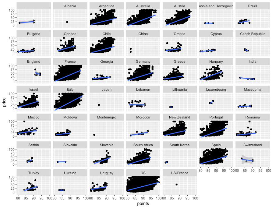
All pictures copied from the GitHub page of ggstatsplot [original]

ggscatterstats

Not all plots are ggplot2-compatible though, for instance, ggscatterstats is not. Nevertheless, it produces a very powerful plot in my opinion.

ggstatsplot::ggscatterstats(
  data = datasets::iris, 
  x = Sepal.Length, 
  y = Petal.Length,
  title = "Dataset: Iris flower data set",
  messages = FALSE
)
All pictures copied from the GitHub page of ggstatsplot [original]

ggcormat

ggcorrmat is also quite impressive, producing correlalograms with only minimal amounts of code as it wraps around ggcorplot. The defaults already produces publication-ready correlation matrices:

ggstatsplot::ggcorrmat(
  data = datasets::iris,
  corr.method = "spearman",
  sig.level = 0.005,
  cor.vars = Sepal.Length:Petal.Width,
  cor.vars.names = c("Sepal Length", "Sepal Width", "Petal Length", "Petal Width"),
  title = "Correlalogram for length measures for Iris species",
  subtitle = "Iris dataset by Anderson",
  caption = expression(
    paste(
      italic("Note"),
      ": X denotes correlation non-significant at ",
      italic("p "),
      "< 0.005; adjusted alpha"
    )
  )
)
All pictures copied from the GitHub page of ggstatsplot [original]

ggcoefstats

Finally, ggcoefstats is a wrapper around GGally::ggcoef, creating a plot with the regression coefficients’ point estimates as dots with confidence interval whiskers. Here’s an example with some detailed specifications:

ggstatsplot::ggcoefstats(
  x = stats::lm(formula = mpg ~ am * cyl,
                data = datasets::mtcars),
  point.color = "red",
  vline.color = "#CC79A7",
  vline.linetype = "dotdash",
  stats.label.size = 3.5,
  stats.label.color = c("#0072B2", "#D55E00", "darkgreen"),
  title = "Car performance predicted by transmission and cylinder count",
  subtitle = "Source: 1974 Motor Trend US magazine"
) +                                    
  ggplot2::scale_y_discrete(labels = c("transmission", "cylinders", "interaction")) +
  ggplot2::labs(x = "regression coefficient",
                y = NULL)

All pictures copied from the GitHub page of ggstatsplot [original]
I for one am very curious to see how Indrajeet will further develop this package, and whether academics will start using it as a default in publishing.


Generating Book Covers By Their Words — My Dissertation Cover

Generating Book Covers By Their Words — My Dissertation Cover

As some of you might know, I am defending my PhD dissertation later this year. It’s titled “Data-Driven Human Resource Management: The rise of people analytics and its application to expatriate management” and, over the past few months, I was tasked with designing its cover.

Now, I didn’t want to buy some random stock photo depicting data, an organization, or overly happy employees. I’d rather build something myself. Something reflecting what I liked about the dissertation project: statistical programming and sharing and creating knowledge with others.

Hence, I came up with the idea to use the collective intelligence of the People Analytics community to generate a unique cover. It required a dataset of people analytics-related concepts, which I asked People Analytics professionals on LinkedIn, Twitter, and other channels to help compile. Via a Google Form, colleagues, connections, acquitances, and complete strangers contributed hundreds of keywords ranging from the standard (employees, HRM, performance) to the surprising (monetization, quantitative scissors [which I had to Google]). After reviewing the list and adding some concepts of my own creation, I ended up with 1786 unique words related to either business, HRM, expatriation, data science, or statistics.

I very much dislike wordclouds (these are kind of cool though), but already had a different idea in mind. I thought of generating a background cover of the words relating to my dissertation topic, over which I could then place my title and other information. I wanted to place these keywords randomly, maybe using a color schema, or with some random sizes.

The picture below shows the result of one of my first attempts. I programmed everything in R, writing some custom functionality to generate the word-datasets, the cover-plot, and .png, .pdf, and .gif files as output.

canvas.PNG

Random colors did not produce a pleasing result and I definitely needed more and larger words in order to fill my 17cm by 24cm canvas!

Hence, I started experimenting. Using base R’s expand.grid() and set.seed() together with mapply(), I could quickly explore and generate a large amount of covers based on different parameter settings and random fluctuations.

expand.grid(seed = c(1:3), 
            dupl = c(1:4, seq(5, 30, 5)),
            font = c("sans", "League Spartan"),
            colors = c(blue_scheme, red_scheme, 
                       rainbow_scheme, random_scheme),
            size_mult = seq(1, 3, 0.3),
            angle_sd = c(5, 10, 12, 15)) -> 
  param

mapply(create_textcover, 
       param$seed, param$dupl, 
       param$font, param$colors, 
       param$size_mult, param$angle_sd)

The generation process for each unique cover only took a few seconds, so I would generate a few hundred, quickly browse through them, update the parameters to match my preferences, and then generate a new set. Among others, I varied the color palette used, the size range of the words, their angle, the font used, et cetera. To fill up the canvas, I experimented with repeating the words: two, three, five, heck, even twenty, thirty times. After an evening of generating and rating, I came to the final settings for my cover:

  • Words were repeated twenty times in the dataset.
  • Words were randomly distributed across the canvas.
  • Words placed in random order onto the canvas, except for a select set of relevant words, placed last.
  • Words’ transparency ranged randomly between 0% and 70%.
  • Words’ color was randomly selected out of six colors from this palette of blues.
  • Words’ writing angles were normally distributed around 0 degrees, with a standard deviation of 12 degrees. However, 25% of words were explicitly without angle.
  • Words’ size ranged between 1 and 4 based on a negative binomial distribution (10 * 0.8) resulting in more small than large words. The set of relevant words were explicitly enlarged throughout.

With League Spartan (#thisisparta) loaded as a beautiful custom font, this was the final cover background which I and my significant other liked most:

cover_wordcloud_20-League Spartan-4.png

While I still need to decide on the final details regarding title placement and other details, I suspect that the final cover will look something like below — the white stripe in the middle depicting the book’s back.

coverpaul.png

Now, for the finale, I wanted to visualize the generation process via a GIF. Thomas Lin Pedersen developed this great gganimate package, which builds on the older animation package. The package greatly simplifies creating your own GIFs, as I already discussed in this earlier blog about animated GIFs in R. Anywhere, here is the generation process, where each frame includes the first frame ^ 3.2 words:

cover_wordcloud_20-League Spartan_4.gif

If you are interested in the process, or the R code I’ve written, feel free to reach out!

I’m sharing a digital version of the dissertation online sometime around the defense date: November 9th, 2018. If you’d like a copy, you can still leave your e-mailadress in the Google Form here and I’ll make sure you’ll receive your copy in time!

Become a data-driven Sommelier by text mining wine reviews

Become a data-driven Sommelier by text mining wine reviews

Aleszu Bajak at Storybench.org published a great demonstration of the power of text mining. He used the R tidytext package to analyse 150,000 wine reviews which Zach Thoutt had scraped from Wine Enthusiast in November of 2017.

Aleszu started his analysis on only the French wines, with a simple word count per region:

[orginal blog]
Next, he applied TF-IDF to surface the words that are most characteristic for specific French wine regions — words used often in combination with that specific region, but not in relation to other regions.

[orginal blog]
The data also contained some price information, which Aleszu mapped France with ggplot2 and the maps package to demonstrate which French wine regions are generally more costly.

[orginal blog]
On the full dataset, Alezsu also demonstrated that there is a strong relationship between price and points, meaning that, in general, more expensive wines seem to get better reviews:

[orginal blog]
The full script and more details you can find in the orginal blog.

Sentiment Analysis of Stranger Things Seasons 1 and 2

Sentiment Analysis of Stranger Things Seasons 1 and 2

Jordan Dworkin, a Biostatistics PhD student at the University of Pennsylvania, is one of the few million fans of Stranger Things, a 80s-themed Netflix series combining drama, fantasy, mystery, and horror. Awaiting the third season, Jordan was curious as to the emotional voyage viewers went through during the series, and he decided to examine this using a statistical approach. Like I did for the seven Harry Plotter books, Jordan downloaded the scripts of all the Stranger Things episodes and conducted a sentiment analysis in R, of course using the tidyverse and tidytext. Jordan measured the positive or negative sentiment of the words in them using the AFINN dictionary and a first exploration led Jordan to visualize these average sentiment scores per episode:

The average positive/negative sentiment during the 17 episodes of the first two seasons of Stranger Things (from Medium.com)

Jordan jokingly explains that you might expect such overly negative sentiment in show about missing children and inter-dimensional monsters. The less-than-well-received episode 15 stands out, Jordan feels this may be due to a combination of its dark plot and the lack of any comedic relief from the main characters.

Reflecting on the visual above, Jordan felt that a lot of the granularity of the actual sentiment was missing. For a next analysis, he thus calculated a rolling average sentiment during the course of the separate episodes, which he animated using the animation package:

GIF displaying the rolling average (40 words) sentiment per Stranger Things episode (from Medium.com)

Jordan has two new takeaways: (1) only 3 of the 17 episodes have a positive ending – the Season 1 finale, the Season 2 premiere, and the Season 2 finale – (2) the episodes do not follow a clear emotional pattern. Based on this second finding, Jordan subsequently compared the average emotional trajectories of the two seasons, but the difference was not significant:

Smoothed (loess, I guess) trajectories of the sentiment during the episodes in seasons one and two of Stranger Things (from Medium.com)

Potentially, it’s better to classify the episodes based on their emotional trajectory than on the season they below too, Jordan thought next. Hence, he constructed a network based on the similarity (temporal correlation) between episodes’ temporal sentiment scores. In this network, the episodes are the nodes whereas the edges are weighted for the similarity of their emotional trajectories. In that sense, more distant episodes are less similar in terms of their emotional trajectory. The network below, made using igraph (see also here), demonstrates that consecutive episodes (1 → 2, 2 → 3, 3 → 4) are not that much alike:

The network of Stranger Things episodes, where the relations between the episodes are weighted for the similarity of their emotional trajectories (from Medium.com).

A community detection algorithm Jordan ran in MATLAB identified three main trajectories among the episodes:

Three different emotional trajectories were identified among the 17 Stranger Things episodes in Season 1 and 2 (from Medium.com).

Looking at the average patterns, we can see that group 1 contains episodes that begin and end with neutral emotion and have slow fluctuations in the middle, group 2 contains episodes that begin with negative emotion and gradually climb towards a positive ending, and group 3 contains episodes that begin on a positive note and oscillate downwards towards a darker ending.

– Jordan on Medium.com

Jordan final suggestion is that producers and scriptwriters may consciously introduce these variations in emotional trajectories among consecutive episodes in order to get viewers hooked. If you want to redo the analysis or reuse some of the code used to create the visuals above, you can access Jordan’s R scripts here. I, for one, look forward to his analysis of Season 3!

Functional programming and why not to “grow” vectors in R

Functional programming and why not to “grow” vectors in R

For fresh R programmers, vectorization can sound awfully complicated. Consider two math problems, one vectorized, and one not:

math_operations.png
Two ways of doing the same computations in R

Why on earth should R spend more time calculating one over the other? In both cases there are the same three addition operations to perform, so why the difference? This is what we will try to illustrate in this post, which is inspired on work by Naom Ross and the University of Auckland.

R behind the scenes:

R is a high-levelinterpreted computer language. This means that R takes care of a lot of basic computer tasks for you. For instance, when you type i <- 5.0 you don’t have to tell R:

  • That 5.0 is a floating-point number
  • That i should store numeric-type data
  • To find a place in memory for to put 5
  • To register i as a pointer to that place in memory

You also don’t have to convert i <- 5.0 to binary code. That’s done automatically when you hit Enter. Although you are probably not aware of this, many R functions are just wrapping your input and passing it to functions of other, compiled computer languages, like C, C++, or FORTRAN, in the back end.

Now here’s the crux: If you need to run a function over a set of values, you can either pass in a vector of these values through the R function to the compiled code (math example 1), or you could call the R function repeatedly for each value separately (math example 2). If you do the latter, R has to do stuff (figuring out the above bullet points and translating the codeeach time, repeatedly. However, if you call the function with a vector instead, this figuring out part only happens once. For instance, R vectors are constricted to a single data type (e.g., numeric, character) and when you use a vector instead of seperate values, R only needs to determine the input data type once, which saves time. In short, there’s no advantage to NOT organizing your data as vector.

For-loops and functional programming (*ply)

One example of how new R programmers frequently waste computing time is via memory allocation. Take the below for loop, for instance:

iterations = 10000000
 
 system.time({
   j = c()
   for(i in 1:iterations){
     j[i] <- i
   }
 })
##    user  system elapsed 
##    3.71    0.23    3.94

Here, vector j starts out with length 1, but for each iteration in the for loop, R has to re-size the vector and re-allocate memory. Recursively, R has to find the vector in its memory, create a new vector that will fit more data, copy the old data over, insert the new data, and erase the old vector. This process gets very slow as vectors get big. Nevertheless, it is often how programmers store the results of their iterative processes. Tremendous computing power can be saved by pre-allocating vectors to fit all the values beforehand, so that R does not have to do unnecessary actions:

system.time({
   j = rep(NA, iterations)
   for(i in 1:iterations){
     j[i] <- i
   }
 })
##    user  system elapsed 
##    0.88    0.01    0.89

More advanced R users tend to further optimize via functionals. This family of functions takes in vectors (or matrices, or lists) of values and applies other functions to each. Examples are apply or plyr::*ply functions, which speed up R code mainly because the for loops they have inside them automatically do things like pre-allocating vector size. Functionals additionally prevent side effects: unwanted changes to your working environment, such as the remaining i after for(i in 1:10). Although this does not necessarily improve computing time, it is regarded best practice due to preventing consequent coding errors.

Conclusions

There are cases when you should use for loops. For example, the performance penalty for using a for loop instead a vector will be small if the number of iterations is relatively small, and the functions called inside your for loop are slow. Here, looping and overhead from function calls make up a small fraction of your computational time and for loops may be more intuitive or easier to read for you. Additionally, there are cases where for loops make more sense than vectorized functions: (1) when the functions you seek to apply don’t take vector arguments and (2) when each iteration is dependent on the results of previous iterations.

Another general rule: fast R code is short. If you can express what you want to do in R in a line or two, with just a few function calls that are actually calling compiled code, it’ll be more efficient than if you write long program, with the added overhead of many function calls.

Finally, there is a saying that “premature optimization is the root of all evil”. What this means is that you should not re-write your R code unless the computing time you are going to save is worth the time invested. Nevertheless, if you understand how vectorization and functional programming work, you will be able to write more faster, safer, and more transparent (short & simple) programs.